Reading a RMarkdown Script

What is a script?

Scripts are files that:

Record and organize a sequence of commands in a logical manner
Facilitate running many commands in rapid succession
Help to reproduce and share your work with others

While it is possible to enter and run commands directly from the R Console, scripts will be the default way to work.

If you are more familiar with Stata, a script is equivalent to a Do File.

Remember to save your script as you work!

What is a RMarkdown Script?

RMarkdown scripts can contain commands such as for data import, cleaning, etc. and are themselves the outline of an automatically-generated document containing text, tables, and plots produced by your code.

You can learn more about RMarkdown here and reference this cheatsheet

In the above RMarkdown template script, the white and gray code chunks produce text and R-generated graphics, respectively, in the Word document report. The green text does not appear in the final report.

Understand a RMarkdown

Code chunks

While the RMarkdown may at first look like a wall of code, notice how “chunks” of code are differentiated by their color:

In WHITE background areas, any text will appear as regular text in the final report.
- Can have formatting such as headings, italics, bold, numbers, and bullets. See the second page of this RMarkdown cheatsheet for more detail.
- Can display parameters derived from your data via in-line code (such as epi week of the outbreak peak, as in the example above).
In GRAY background “code chunks”, RMarkdown is running R commands. These commands perform data processing and cleaning steps, or could produce visual outputs in the document.
GREEN text in the RMarkdown will not appear in the final report. These sections, placed between special characters (known as html comment tags, ), serve as instructions for you.


<!-- ~~~~~~~~~~~~~~~~~~~~~~~~~~~~~~~~~~~~~~~~~~~~~~~~~~~~~~~~~~~~~~~~~~~~~~~~~~~
This comment will not show up when you knit the document.
A comment with a title with slashes indicates a name of a code chunk.
~~~~~~~~~~~~~~~~~~~~~~~~~~~~~~~~~~~~~~~~~~~~~~~~~~~~~~~~~~~~~~~~~~~~~~~~~~~~ -->

Navigating the RMarkdown

Use the Table of Contents menu in the bottom-left of the script to easily navigate between code chunks and sections of the script. The line numbers on the left side can be helpful to reference specific commands when asking for assistance.

Running code chunks

While editing and testing your RMarkdown, you may want to selectively run or re-run R code chunks. You have many options in the script’s Run menu, including:

Run specific code within a chunk
Run one R code chunk at a time
Run all R code chunks above or below the selected chunk

Progress bars and previews of chunk output/error messages help with revisions and trouble-shooting.

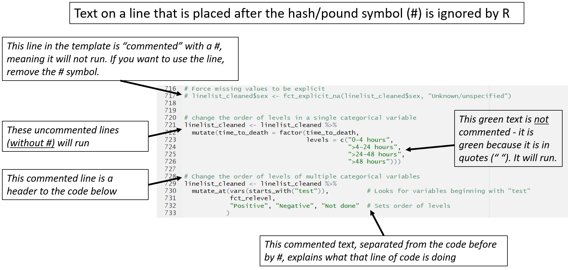
Commented code

Every script should include helpful text that organizes commands and explains their rationale to collaborators. The # (hash or comment) symbol ensures that any text after the # and on the same line will not be executed by R as it runs the script. Such “commented” text will appear a different color than the code.

In the templates, you will see # serving three purposes:

# Explanatory text or section headers with an R chunk. This commented text can be placed after code, or in the line above.

# An example of commented text  
linelist_raw <- gen_data("AJS") # generates a fake dataset for use in this template

# Optional commands that can be uncommented as needed. For example, you can uncomment and run the last line below if your dataset meets the relevant criteria.

# If your linelist is a csv export of data from DHIS2 use this code chunk
# This assumes your data fits the standardised MSF data dictionary for this disease

## Read data ------------------------------------------------------
# CSV file
# linelist_raw <- rio::import("linelist.csv")

### As section titles. In the plain text sections of the RMarkdown script (not R code chunks), hash/comment symbols produce titles and section headers.

Multiple lines of R code can be commented/uncommented by highlighting the lines and pressing the keys Ctrl, Shift, and C at the same time (Ctrl+Shift+C).

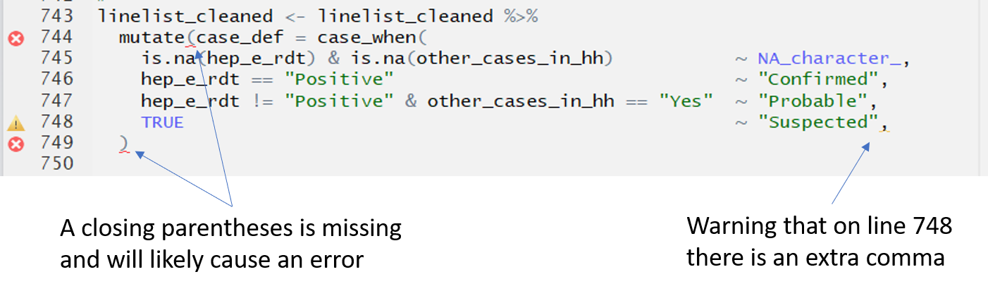
Code assists

Any script (RMarkdown or otherwise) will give clues when you have made a mistake. For example, if you forgot to write a comma where it is needed, or to close a parentheses, RStudio will raise a flag on that line, on the right side of the script, to warn you.

Producing/“Knitting” the RMarkdown document

Producing the final RMarksdown report is called “knitting”. When you are editing a RMarkdown script, you will see a special option to “Knit”" at the top of the script, near the save shortcut button. Clicking “Knit” will begin the process of creating the final document. The option to “Knit” does not appear for normal R scripts, only RMarkdown scripts. Note the following:

You can use the arrow next to the word “Knit” to select the type of document you want to produce: Microsoft Word, PDF, or HTML (HTML opens the file in an offline web browser). Note that to knit to a PDF directly, additional packages may have to be installed.
The default document type is specified in the header of the RMarkdown script, and for the templates it is Microsoft Word.

If you receive an error when knitting such as “openBinaryFile does not exist … Error: pandoc document conversion failed with error 1”, your R project file may be saved in a location with restricted permissions such as a network drive. The RMarkdown is likely not permitted to write the new Microsoft Word file to that location. Try saving your R project to a more local location on your computer.

If you are on an MSF computer, try writing saving the R project on the C drive where you have read/write rights - in general this is the c:temp folder.