Person analyses
After cleaning the data, there are three sections of the template that produce tabular, graphic, and cartographic (map) analysis outputs.
This first section produces descriptive analyses about the patients demographics and attack rates.
Demographic Tables:
The person analysis section begins with a couple sentences that contain in-line code - code embedded in normal RMarkdown text (not within an R code chunk). The second sentence in-line code inserts the number of males and females by counting the observations with “Male” and “Female” in the variable sex. Because our dataset’s variable sex contains M and F instead, we must modify this in-line code (or modify our variable) so the fmt_count() function is searching for the correct terms.
The first demographic table presents patients by their age group (the table’s rows) and their relationship with the case definition (the table’s columns). This chunk uses piping to link six different functions and produce a table (%>% is the pipe operator - see the R Basics Advanced and Miscellaneous page):
- The
tab_linelist()function creates a frequency and percent table ofage_group, with columns differentiating bycase_defvalue
- The
select()function removes an unnecessary column “variable” generated bytab_linelist().
- The
rename()function renames the default column “value” as “Age Group”
- The
rename_redundant()function replaces any column name that has proportion with “%”
- The
augment_redundant()command replaces any column name with n with " cases (n)"
- The
kable()command completes the table, in this case with one digit after each decimal
# Describe observations by age_group and case_def
tab_linelist(linelist_cleaned,
             age_group, strata = case_def,
             col_total = TRUE, row_total = TRUE) %>%
  select(-variable) %>%
  rename("Age group" = value) %>%
  rename_redundant("%" = proportion) %>%
  augment_redundant(" cases (n)" = " n$") %>%
kable(digits = 1)| Age group | Confirmed cases (n) | % | Probable cases (n) | % | Suspected cases (n) | % | Missing cases (n) | % | Total |
|---|---|---|---|---|---|---|---|---|---|
| 0-2 | 4 | 4.0 | 0 | 0.0 | 40 | 5.8 | 23 | 3.7 | 67 |
| 3-14 | 30 | 30.3 | 1 | 16.7 | 284 | 40.9 | 320 | 50.9 | 635 |
| 15-29 | 46 | 46.5 | 2 | 33.3 | 246 | 35.4 | 180 | 28.6 | 474 |
| 30-44 | 15 | 15.2 | 2 | 33.3 | 95 | 13.7 | 76 | 12.1 | 188 |
| 45+ | 4 | 4.0 | 1 | 16.7 | 29 | 4.2 | 30 | 4.8 | 64 |
| Total | 99 | 100.0 | 6 | 100.0 | 694 | 100.0 | 629 | 100.0 | 1428 |
You can change the argument strata = to refer to any number of variables (in this next example, sex). To show proportions of the total population of observations, add the argument prop_total = specified as TRUE, as below.
tab_linelist(linelist_cleaned,
             age_group, strata = sex,
             col_total = TRUE, row_total = TRUE, prop_total = TRUE) %>%
  select(-variable) %>%
  rename("Age group" = value) %>%
#  rename_redundant("%" = proportion) %>%
  augment_redundant(" cases (n)" = " n$") %>%
kable(digits = 1)| Age group | F cases (n) | F proportion | M cases (n) | M proportion | Total |
|---|---|---|---|---|---|
| 0-2 | 26 | 1.8 | 41 | 2.9 | 67 |
| 3-14 | 222 | 15.5 | 413 | 28.9 | 635 |
| 15-29 | 316 | 22.1 | 158 | 11.1 | 474 |
| 30-44 | 118 | 8.3 | 70 | 4.9 | 188 |
| 45+ | 32 | 2.2 | 32 | 2.2 | 64 |
| Total | 714 | 50.0 | 714 | 50.0 | 1428 |
You can also choose to exclude or edit the in-line code that gives a count of the missing cases by sex and age_group.
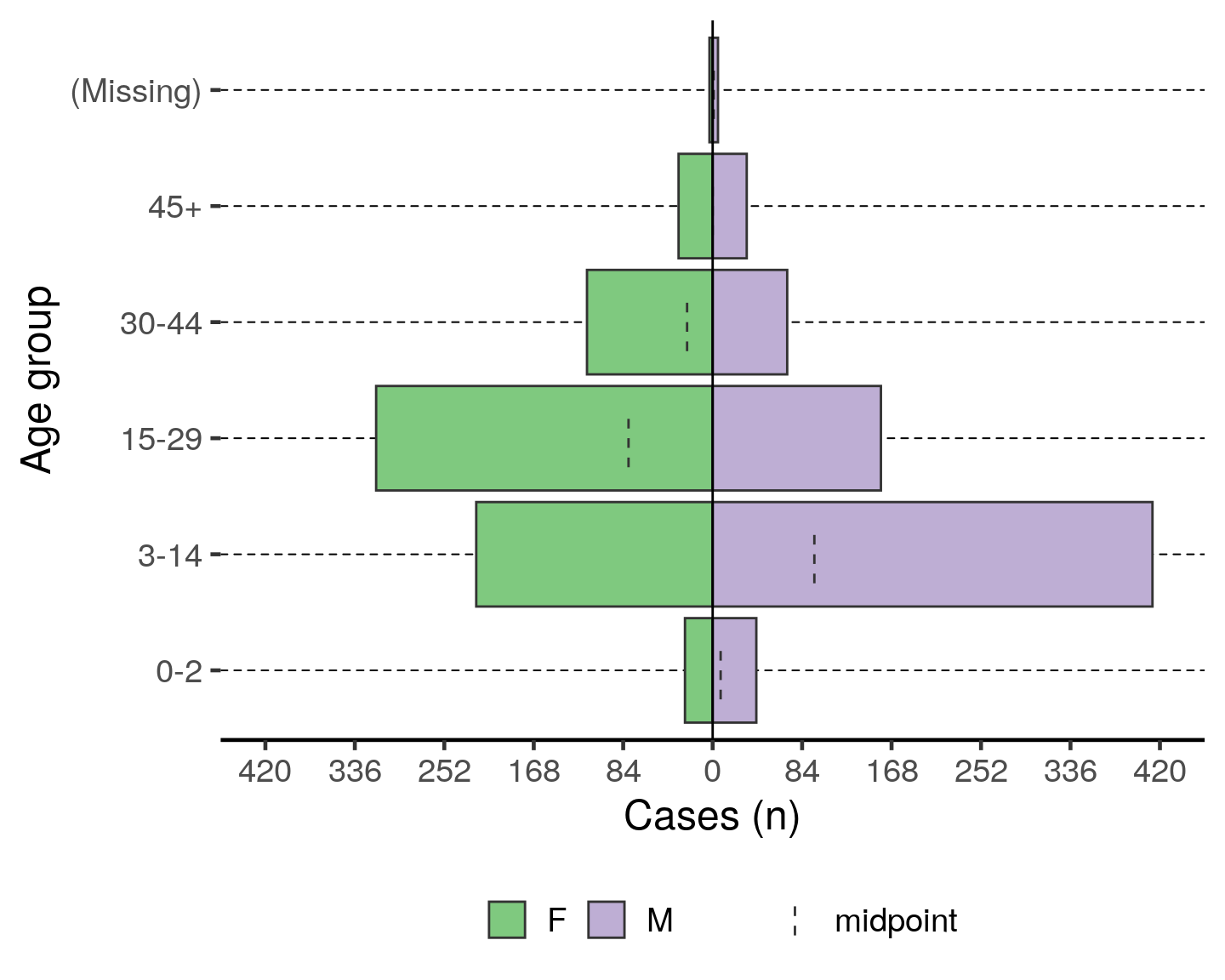
Age pyramids
To print an age pyramid in your report, use the code below. A few things to note:
- The variable for
split_by =should have two non-missing value options (e.g. Male or Female, Oui or Non, etc. Three will create a messy output.)
- The variable names work with or without quotation marks
- The dashed lines in the bars are the midpoint of the un-stratified age group
- You can adjust the position of the legend by replacing
legend.position = "bottom"with “top”, “left”, or “right”
- Read more by searching “plot_age_pyramid”" in the Help tab of the lower-right RStudio pane
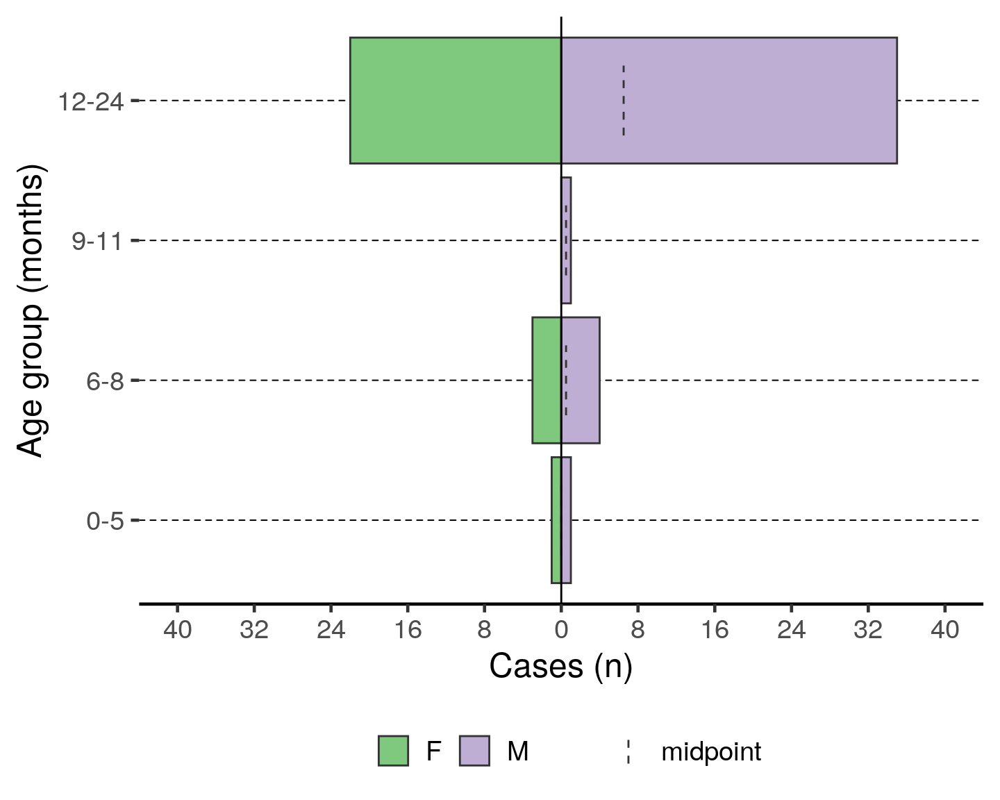
You can make this a pyramid of months by supplying age_group_mon to the age_group = argument.
# plot age pyramid by sex
plot_age_pyramid(linelist_cleaned,
                 age_group = "age_group",
                 split_by = "sex") +
  labs(y = "Cases (n)", x = "Age group") + # change axis  labels (nb. x/y flip)
  theme(legend.position = "bottom",     # move legend to bottom
        legend.title = element_blank(), # remove title
        text = element_text(size = 18)  # change text size
       )
To have an age pyramid of patients under 2 by month age groups, it is best to add a filter() step to the beginning of the code chunk, as below. This selects for linelist_cleaned observations that meet the specified critera and passes that reduced dataset through the “pipes” to the next function: (plot_age_pyramid()). If this filter() step is not added, you will see that the largest pyramid bars are of “missing”. These are the patients old enough to not have a months age group.
If you add this filtering step, you must also modify plot_age_pyramid() by removing its first argument linelist_cleaned,. The dataset is already given to the command in the filter() and is passed to plot_age_pyramid() via piping.
Note that the filter step does not drop any observations from the linelist_cleaned object itself. Because the filter is not being assigned (<-) to over-write linelist_cleaned, this filter is only temporarily applied for the purpose of producing the age pyramid.
# plot age pyramid by month groups, for observations under 2 years
filter(linelist_cleaned, age_years <= 2) %>%
  plot_age_pyramid(age_group = "age_group_mon",
                   split_by = "sex") +
                  # stack_by = "case_def") +
  labs(y = "Cases (n)", x = "Age group (months)") + # change axis  labels (nb. x/y flip)
  theme(legend.position = "bottom",     # move legend to bottom
        legend.title = element_blank(), # remove title
        text = element_text(size = 18)  # change text size
       )
Inpatient statistics
The text following the age pyramids uses in-line code to describe the distribution of outpatient and inpatient observations, and descriptive statistics of the length of stay for inpatients. The Am Timan dataset does not have length of stay, so it is best to delete those related sentences related to obs_days for the final report.
Symptom and lab descriptive tables
This next code also uses the tab_linelist() function to create descriptive tables of all the variables that were included in the SYMPTOMS variable list.
- In the
tab_linelist()function,SYMPTOMS(the value supplied to the second argument) is an object we defined in data cleaning that is a list of variables to tabulate. If this code produces an error about an “Unknown column”, ensure that the variables in the objectSYMPTOMSare all present in your dataset (and spelled correctly). - Also in
tab_linelist(), the argumentkeep =must represent the character value to be counted for the the table. As these Am Timan variables are still in French, we changekeep = "Yes"tokeep = "Oui".
- The
mutate()function is aesthetically changing variable names with underscores to spaces.
# get counts and proportions for all variables named in SYMPTOMS
tab_linelist(linelist_cleaned, SYMPTOMS, keep = "Oui") %>%
  select(-value) %>%
  # fix the way symptom names are displayed
  mutate(variable = str_to_sentence(str_replace_all(variable, "_", " "))) %>%
  # rename accordingly
  rename_redundant("%" = proportion) %>%
  augment_redundant(" (n)" = " n$") %>%
kable(digits = 1)| variable | n | % |
|---|---|---|
| Generalized itch | 512 | 64.6 |
| Fever | 668 | 84.0 |
| Joint pains | 240 | 30.5 |
| Epigastric pain heartburn | 469 | 59.2 |
| Nausea anorexia | 425 | 53.5 |
| Vomiting | 457 | 57.6 |
| Diarrhoea | 112 | 14.2 |
| Bleeding | 52 | 6.6 |
| Headache | 633 | 80.0 |
The code for the lab table is very similar, but has this difference:
- In the initial
tab_linelist()command,transpose = "value"is set because the values in the lab data are important in-and-of themselves (e.g. IgM+/IgG-, etc.) - i.e. the values should become column headers.
This table may be large and unwieldy at first, until you clean your data. The step in data cleaning where we converted 0, 1, “yes”, “pos”, “neg”, etc. to standardized “Positive” and “Negative” was crucial towards making this table readable. Once knitted into a word document, you will likely need to adjust the font size, column widths, etc.
# get counts and proportions for all variables named in LABS
tab_linelist(linelist_cleaned, LABS,
             transpose = "value") %>%
  # fix the way lab test names are displayed
  mutate(variable = str_to_sentence(str_replace_all(variable, "_", " "))) %>%
  # rename accordingly
  rename("Lab test" = variable) %>%
  rename_redundant("%" = proportion) %>%
  augment_redundant(" (n)" = " n$") %>%
kable(digits = 1)| Lab test | Negative (n) | % | Positive (n) | % | IgG-/IgM- (n) | % | IgG-/IgM+ (n) | % | IgG+/IgM- (n) | % | IgG+/IgM+ (n) | % | IgG±/IgM- (n) | % |
|---|---|---|---|---|---|---|---|---|---|---|---|---|---|---|
| Hep b rdt | 222 | 91.7 | 20 | 8.3 | - | - | - | - | - | - | - | - | - | - |
| Hep c rdt | 239 | 99.2 | 2 | 0.8 | - | - | - | - | - | - | - | - | - | - |
| Hep e rdt | 149 | 59.8 | 100 | 40.2 | - | - | - | - | - | - | - | - | - | - |
| Test hepatitis a | 23 | 100.0 | - | - | - | - | - | - | - | - | - | - | - | - |
| Test hepatitis b | 22 | 95.7 | 1 | 4.3 | - | - | - | - | - | - | - | - | - | - |
| Test hepatitis c | 23 | 100.0 | - | - | - | - | - | - | - | - | - | - | - | - |
| Test hepatitis e igm | 21 | 33.9 | 41 | 66.1 | - | - | - | - | - | - | - | - | - | - |
| Test hepatitis e genotype | - | - | 2 | 100.0 | - | - | - | - | - | - | - | - | - | - |
| Test hepatitis e virus | 7 | 11.3 | 1 | 1.6 | 9 | 14.5 | 14 | 22.6 | 5 | 8.1 | 26 | 41.9 | - | - |
| Malaria rdt at admission | 160 | 63.5 | 92 | 36.5 | - | - | - | - | - | - | - | - | - | - |
| Dengue | - | - | - | - | 12 | 52.2 | - | - | 10 | 43.5 | - | - | 1 | 4.3 |
| Yellow fever | - | - | - | - | 18 | 78.3 | - | - | 5 | 21.7 | - | - | - | - |
| Chikungunya onyongnyong | - | - | - | - | 20 | 87.0 | - | - | 3 | 13.0 | - | - | - | - |
| Other arthropod transmitted virus | 23 | 100.0 | - | - | - | - | - | - | - | - | - | - | - | - |
Case Fatality Ratio (CFR)
The opening text of this chunk with in-line code must be edited to match our Am Timan data. The second in-line code references the variable exit_status - this must now reference the variable exit_status2. Also, we do not have Dead on Arrival recorded in our dataset, so that part of the sentence should be deleted.
Likewise, the code section on time-to-death does not apply to our dataset and should be deleted.
Overall CFR is produced with the code below. Note the following:
- This code requires the variable
patient_facility_type, that it has a value “Inpatient”, and theDIEDvariable.
- A filter is applied that restricts this table to Inpatient observations only.
rename()is used to change the column labels in the table
# use arguments from above to produce overal CFR
overall_cfr <- linelist_cleaned %>%
  filter(patient_facility_type == "Inpatient") %>%
  case_fatality_rate_df(deaths = DIED, mergeCI = TRUE) %>%
  rename("Deaths" = deaths,
         "Cases" = population,
         "CFR (%)" = cfr,
         "95%CI" = ci)
knitr::kable(overall_cfr, digits = 1) # print nicely with 1 decimal digit| Deaths | Cases | CFR (%) | 95%CI |
|---|---|---|---|
| 13 | 86 | 15.1 | (9.05–24.16) |
The next code adds arguments to case_fatality_rate_df() such as group = sex (which stratified the CFR by sex), and add_total = TRUE (which makes a total row across the sex groups).
linelist_cleaned %>%
  filter(patient_facility_type == "Inpatient") %>%
  mutate(sex = forcats::fct_explicit_na(sex, "-")) %>%
  case_fatality_rate_df(deaths = DIED, group = sex, mergeCI = TRUE, add_total = TRUE) %>%
  rename("Sex" = sex,
         "Deaths" = deaths,
         "Cases" = population,
         "CFR (%)" = cfr,
         "95%CI" = ci) %>%
knitr::kable(digits = 1)| Sex | Deaths | Cases | CFR (%) | 95%CI |
|---|---|---|---|---|
| F | 11 | 55 | 20.0 | (11.55–32.36) |
| M | 2 | 31 | 6.5 | (1.79–20.72) |
| Total | 13 | 86 | 15.1 | (9.05–24.16) |
When creating a table of CFR by age groups, one additional step, using the function complete() is required to ensure that all age_group levels are shown even if they have no observations.
linelist_cleaned %>%
  filter(patient_facility_type == "Inpatient") %>%
  case_fatality_rate_df(deaths = DIED, group = age_group, mergeCI = TRUE, add_total = TRUE) %>%
  tidyr::complete(age_group,
                  fill = list(deaths = 0,
                              population = 0,
                              cfr = 0,
                              ci = 0)) %>% # Ensure all levels are represented
  rename("Age group" = age_group,
         "Deaths" = deaths,
         "Cases" = population,
         "CFR (%)" = cfr,
         "95%CI" = ci) %>%
knitr::kable(digits = 1)| Age group | Deaths | Cases | CFR (%) | 95%CI |
|---|---|---|---|---|
| 0-2 | 4 | 11 | 36.4 | (15.17–64.62) |
| 3-14 | 1 | 17 | 5.9 | (1.05–26.98) |
| 15-29 | 5 | 36 | 13.9 | (6.08–28.66) |
| 30-44 | 2 | 17 | 11.8 | (3.29–34.34) |
| 45+ | 1 | 4 | 25.0 | (4.56–69.94) |
| (Missing) | 0 | 1 | 0.0 | (0.00–79.35) |
| Total | 13 | 86 | 15.1 | (9.05–24.16) |
The commented code below examines CFR by case definition. Note that this is dependant upon our working case_def variable.
# Use if you have enough confirmed cases for comparative analysis

 linelist_cleaned %>%
   filter(patient_facility_type == "Inpatient") %>%
   case_fatality_rate_df(deaths = DIED, group = case_def, mergeCI = TRUE, add_total = TRUE) %>%
   rename("Case definition" = case_def,
          "Deaths" = deaths,
          "Cases" = population,
          "CFR (%)" = cfr,
          "95%CI" = ci) %>%
knitr::kable(digits = 1)| Case definition | Deaths | Cases | CFR (%) | 95%CI |
|---|---|---|---|---|
| Confirmed | 8 | 44 | 18.2 | (9.51–31.96) |
| Suspected | 5 | 42 | 11.9 | (5.19–25.00) |
| Total | 13 | 86 | 15.1 | (9.05–24.16) |
Attack Rate
To use the attack rate section, we need to modify the first code slightly. An object population is created from the sum of population counts in the population figures. Because we only imported region-based population counts, we must change this command to reflect that we do not have population_data_age, but rather population_data_region.
# OLD command from template
# population <- sum(population_data_age$population)
Running the correct command and printing the value of population, we see that the sum population across regions is estimated to be 62336.
# CORRECTED command for Am Timan exercise
population <- sum(population_data_region$population)

population
## [1] 62336The first line of code below creates a multi-part object ar with the number of cases, population, attack rate per 10,000, and lower and upper confidence intervals (you can run just this line to verify yourself). The subsequent commands alter the aesthetics of to produce a neat table with appropriate column names.
# calculate the attack rate information and store them in object "ar""
ar <- attack_rate(nrow(linelist_cleaned), population, multiplier = 10000)

# Create table from the information in the object "ar""
ar %>%
  merge_ci_df(e = 3) %>% # merge the lower and upper CI into one column
  rename("Cases (n)" = cases,
         "Population" = population,
         "AR (per 10,000)" = ar,
         "95%CI" = ci) %>%
  select(-Population) %>% # drop the population column as it is not changing
knitr::kable(digits = 1, align = "r")| Cases (n) | AR (per 10,000) | 95%CI |
|---|---|---|
| 1436 | 230.4 | (218.88–242.44) |
We are unable to calculate the attack rate by age group, because we do not have population counts for each age group. Comment out (#) this code.
Mortality attributable to AJS is also not appropriate for this example. Comment out (#) the 4 related code chunks.