Place analyses
The final section of the template produces tabular analysis outputs related to place. If you have shapefiles for your situation, you can also produce maps.
Tabular place analyses (non-maps)
To get a basic descriptive table of cases by region (which in our case was originally the variable quartier from the raw linelist), we use tab_linelist() on the variable patient_origin, with columns by patient_facility_type (inpatient, outpatient, or missing).
# Descriptive table of cases by region and facility type
tab_linelist(linelist_cleaned, patient_origin,
             strata = patient_facility_type,
             col_total = TRUE, row_total = TRUE) %>%
  select(-variable) %>%
  rename("Region" = value) %>%
  rename_redundant("%" = proportion) %>%
  augment_redundant(" (n)" = " n$") %>%
kable(digits = 1)| Region | Inpatient (n) | % | Outpatient (n) | % | Missing (n) | % | Total |
|---|---|---|---|---|---|---|---|
| AB GARA | 0 | 0.0 | 0 | 0.0 | 1 | 0.2 | 1 |
| ABLELAYE | 5 | 6.0 | 1 | 0.1 | 2 | 0.3 | 8 |
| ABOUDEA | 1 | 1.2 | 0 | 0.0 | 0 | 0.0 | 1 |
| ADAMRE | 2 | 2.4 | 22 | 3.2 | 24 | 3.7 | 48 |
| ADJABONA | 0 | 0.0 | 0 | 0.0 | 2 | 0.3 | 2 |
| AFFOUSSE | 1 | 1.2 | 1 | 0.1 | 0 | 0.0 | 2 |
| AL-FRECHE | 1 | 1.2 | 0 | 0.0 | 0 | 0.0 | 1 |
| AL-HOUGNA | 1 | 1.2 | 10 | 1.5 | 10 | 1.5 | 21 |
| AL-MOURA | 1 | 1.2 | 0 | 0.0 | 0 | 0.0 | 1 |
| AL ALAK | 0 | 0.0 | 1 | 0.1 | 0 | 0.0 | 1 |
| AL HOUA | 0 | 0.0 | 0 | 0.0 | 1 | 0.2 | 1 |
| AL KOUCK | 0 | 0.0 | 1 | 0.1 | 0 | 0.0 | 1 |
| AL MIDODIL | 1 | 1.2 | 0 | 0.0 | 0 | 0.0 | 1 |
| ALBAYADI | 1 | 1.2 | 1 | 0.1 | 0 | 0.0 | 2 |
| ALBOUKHASS | 0 | 0.0 | 6 | 0.9 | 6 | 0.9 | 12 |
| ALKASSÉ | 4 | 4.8 | 15 | 2.2 | 5 | 0.8 | 24 |
| AM-DOUMA | 0 | 0.0 | 1 | 0.1 | 0 | 0.0 | 1 |
| AM ASSALA | 0 | 0.0 | 1 | 0.1 | 0 | 0.0 | 1 |
| AM BADARO 1 | 0 | 0.0 | 1 | 0.1 | 0 | 0.0 | 1 |
| AM KIFEO | 1 | 1.2 | 0 | 0.0 | 0 | 0.0 | 1 |
| AMANASISSE | 0 | 0.0 | 1 | 0.1 | 0 | 0.0 | 1 |
| AMBARITE | 0 | 0.0 | 3 | 0.4 | 1 | 0.2 | 4 |
| AMCHOKA | 1 | 1.2 | 0 | 0.0 | 0 | 0.0 | 1 |
| AMDIREDIMAT | 1 | 1.2 | 0 | 0.0 | 0 | 0.0 | 1 |
| AMDJALAT | 0 | 0.0 | 2 | 0.3 | 2 | 0.3 | 4 |
| AMMANASIS | 0 | 0.0 | 0 | 0.0 | 2 | 0.3 | 2 |
| AMSINENE | 3 | 3.6 | 5 | 0.7 | 5 | 0.8 | 13 |
| ANALA | 2 | 2.4 | 2 | 0.3 | 4 | 0.6 | 8 |
| ANFANDOCK | 5 | 6.0 | 26 | 3.8 | 19 | 2.9 | 50 |
| ANGUITEI | 0 | 0.0 | 0 | 0.0 | 1 | 0.2 | 1 |
| ANGUITEYE | 0 | 0.0 | 0 | 0.0 | 1 | 0.2 | 1 |
| ARDO | 3 | 3.6 | 2 | 0.3 | 0 | 0.0 | 5 |
| ATETAL | 0 | 0.0 | 0 | 0.0 | 1 | 0.2 | 1 |
| ATOUA | 1 | 1.2 | 1 | 0.1 | 0 | 0.0 | 2 |
| BADINA | 0 | 0.0 | 1 | 0.1 | 0 | 0.0 | 1 |
| BANDJADID | 0 | 0.0 | 1 | 0.1 | 0 | 0.0 | 1 |
| BAUNE | 1 | 1.2 | 0 | 0.0 | 0 | 0.0 | 1 |
| BIR TAGAL | 0 | 0.0 | 1 | 0.1 | 0 | 0.0 | 1 |
| BRANO | 0 | 0.0 | 1 | 0.1 | 0 | 0.0 | 1 |
| CHATAU | 0 | 0.0 | 0 | 0.0 | 1 | 0.2 | 1 |
| COMMERCANT | 0 | 0.0 | 3 | 0.4 | 15 | 2.3 | 18 |
| COUBO ABNIMIR | 0 | 0.0 | 1 | 0.1 | 0 | 0.0 | 1 |
| DARASALAM | 0 | 0.0 | 26 | 3.8 | 25 | 3.8 | 51 |
| DARWAL | 1 | 1.2 | 0 | 0.0 | 0 | 0.0 | 1 |
| DELEBAE | 1 | 1.2 | 1 | 0.1 | 0 | 0.0 | 2 |
| DIFFIR | 2 | 2.4 | 2 | 0.3 | 0 | 0.0 | 4 |
| DIJEKHINÉ | 1 | 1.2 | 0 | 0.0 | 0 | 0.0 | 1 |
| DILEMA | 3 | 3.6 | 22 | 3.2 | 18 | 2.8 | 43 |
| DINGUESS | 2 | 2.4 | 2 | 0.3 | 3 | 0.5 | 7 |
| DJAMBALBAHAR | 0 | 0.0 | 9 | 1.3 | 6 | 0.9 | 15 |
| DJOGO | 0 | 0.0 | 1 | 0.1 | 0 | 0.0 | 1 |
| GANATIR | 5 | 6.0 | 113 | 16.5 | 102 | 15.6 | 220 |
| GANATIR 1 | 0 | 0.0 | 2 | 0.3 | 7 | 1.1 | 9 |
| GANATIR 2 | 0 | 0.0 | 7 | 1.0 | 5 | 0.8 | 12 |
| GARDOLE | 0 | 0.0 | 1 | 0.1 | 2 | 0.3 | 3 |
| GOURMOUDAY | 0 | 0.0 | 2 | 0.3 | 1 | 0.2 | 3 |
| GOZ-TAMADJA | 1 | 1.2 | 2 | 0.3 | 0 | 0.0 | 3 |
| GOZ DJARAT | 1 | 1.2 | 0 | 0.0 | 0 | 0.0 | 1 |
| GOZ MABILE | 1 | 1.2 | 7 | 1.0 | 11 | 1.7 | 19 |
| GOZ MABILE 2 | 1 | 1.2 | 5 | 0.7 | 8 | 1.2 | 14 |
| GRÉDAÏ | 0 | 0.0 | 1 | 0.1 | 0 | 0.0 | 1 |
| HABILÉ | 0 | 0.0 | 1 | 0.1 | 0 | 0.0 | 1 |
| HARAZA | 1 | 1.2 | 0 | 0.0 | 0 | 0.0 | 1 |
| HILE BARA | 2 | 2.4 | 13 | 1.9 | 5 | 0.8 | 20 |
| HILE ODAA | 0 | 0.0 | 2 | 0.3 | 0 | 0.0 | 2 |
| HIMEDA | 0 | 0.0 | 1 | 0.1 | 0 | 0.0 | 1 |
| IDETER | 0 | 0.0 | 1 | 0.1 | 0 | 0.0 | 1 |
| KACHKACHA | 3 | 3.6 | 1 | 0.1 | 2 | 0.3 | 6 |
| KOUBO AMNIMIRE | 0 | 0.0 | 0 | 0.0 | 3 | 0.5 | 3 |
| MABROUKA | 0 | 0.0 | 0 | 0.0 | 1 | 0.2 | 1 |
| MATAR | 0 | 0.0 | 2 | 0.3 | 2 | 0.3 | 4 |
| MINA | 2 | 2.4 | 3 | 0.4 | 8 | 1.2 | 13 |
| MIRÉKIKE | 1 | 1.2 | 0 | 0.0 | 0 | 0.0 | 1 |
| MIRER | 1 | 1.2 | 0 | 0.0 | 0 | 0.0 | 1 |
| MOURAY | 0 | 0.0 | 1 | 0.1 | 0 | 0.0 | 1 |
| NOUGRA KARO | 0 | 0.0 | 1 | 0.1 | 0 | 0.0 | 1 |
| OUM-ALKHOURA | 0 | 0.0 | 0 | 0.0 | 2 | 0.3 | 2 |
| PEDIS | 0 | 0.0 | 1 | 0.1 | 0 | 0.0 | 1 |
| RASSAFIL CHATEAU | 0 | 0.0 | 0 | 0.0 | 1 | 0.2 | 1 |
| RASSALFIL | 3 | 3.6 | 6 | 0.9 | 2 | 0.3 | 11 |
| RIAD | 3 | 3.6 | 37 | 5.4 | 47 | 7.2 | 87 |
| RIDINA | 0 | 0.0 | 72 | 10.5 | 75 | 11.5 | 147 |
| RIDINA 1 | 0 | 0.0 | 2 | 0.3 | 9 | 1.4 | 11 |
| RIDINA 2 | 0 | 0.0 | 5 | 0.7 | 19 | 2.9 | 24 |
| RIMELIE | 0 | 0.0 | 1 | 0.1 | 0 | 0.0 | 1 |
| SALAMAT | 2 | 2.4 | 22 | 3.2 | 23 | 3.5 | 47 |
| SIHEBA | 1 | 1.2 | 0 | 0.0 | 0 | 0.0 | 1 |
| TARADONA | 2 | 2.4 | 136 | 19.9 | 97 | 14.9 | 235 |
| TARADONA 1 | 1 | 1.2 | 14 | 2.0 | 19 | 2.9 | 34 |
| TARADONA 2 | 5 | 6.0 | 39 | 5.7 | 19 | 2.9 | 63 |
| TARADONA 3 | 1 | 1.2 | 6 | 0.9 | 26 | 4.0 | 33 |
| ZONGO | 0 | 0.0 | 3 | 0.4 | 1 | 0.2 | 4 |
| Total | 83 | 100.0 | 684 | 100.0 | 652 | 100.0 | 1419 |
To get a descriptive table by patient outcome we set strata = exit_status2. We can also restrict the analysis to inpatients only by inserting the function filter() into the first argument of tab_linelist. tab_linelist() expects a data frame for it’s first argument, and it receives the filtered linelist_cleaned - this is an example of “nested”" functions (one function inside another).
# get counts and props of region by outcome among inpatients
# include column and row totals
tab_linelist(filter(linelist_cleaned,
                    patient_facility_type == "Inpatient"),
             patient_origin, strata = exit_status2,
             col_total = TRUE, row_total = TRUE) %>%
  select(-variable) %>%
  rename("Region" = value) %>%
  rename_redundant("%" = proportion) %>%
  augment_redundant(" (n)" = " n$") %>%
kable(digits = 1)| Region | Dead (n) | % | Discharged (n) | % | Left (n) | % | Missing (n) | % | Total |
|---|---|---|---|---|---|---|---|---|---|
| ABLELAYE | 1 | 7.7 | 4 | 7.8 | 0 | 0 | 0 | 0.0 | 5 |
| ABOUDEA | 0 | 0.0 | 1 | 2.0 | 0 | 0 | 0 | 0.0 | 1 |
| ADAMRE | 0 | 0.0 | 0 | 0.0 | 1 | 50 | 1 | 5.9 | 2 |
| AFFOUSSE | 0 | 0.0 | 1 | 2.0 | 0 | 0 | 0 | 0.0 | 1 |
| AL-FRECHE | 0 | 0.0 | 1 | 2.0 | 0 | 0 | 0 | 0.0 | 1 |
| AL-HOUGNA | 1 | 7.7 | 0 | 0.0 | 0 | 0 | 0 | 0.0 | 1 |
| AL-MOURA | 0 | 0.0 | 1 | 2.0 | 0 | 0 | 0 | 0.0 | 1 |
| AL MIDODIL | 0 | 0.0 | 1 | 2.0 | 0 | 0 | 0 | 0.0 | 1 |
| ALBAYADI | 0 | 0.0 | 1 | 2.0 | 0 | 0 | 0 | 0.0 | 1 |
| ALKASSÉ | 0 | 0.0 | 4 | 7.8 | 0 | 0 | 0 | 0.0 | 4 |
| AM KIFEO | 0 | 0.0 | 1 | 2.0 | 0 | 0 | 0 | 0.0 | 1 |
| AMCHOKA | 0 | 0.0 | 1 | 2.0 | 0 | 0 | 0 | 0.0 | 1 |
| AMDIREDIMAT | 0 | 0.0 | 1 | 2.0 | 0 | 0 | 0 | 0.0 | 1 |
| AMSINENE | 1 | 7.7 | 0 | 0.0 | 0 | 0 | 2 | 11.8 | 3 |
| ANALA | 0 | 0.0 | 0 | 0.0 | 1 | 50 | 1 | 5.9 | 2 |
| ANFANDOCK | 1 | 7.7 | 4 | 7.8 | 0 | 0 | 0 | 0.0 | 5 |
| ARDO | 0 | 0.0 | 2 | 3.9 | 0 | 0 | 1 | 5.9 | 3 |
| ATOUA | 0 | 0.0 | 1 | 2.0 | 0 | 0 | 0 | 0.0 | 1 |
| BAUNE | 0 | 0.0 | 1 | 2.0 | 0 | 0 | 0 | 0.0 | 1 |
| DARWAL | 0 | 0.0 | 1 | 2.0 | 0 | 0 | 0 | 0.0 | 1 |
| DELEBAE | 1 | 7.7 | 0 | 0.0 | 0 | 0 | 0 | 0.0 | 1 |
| DIFFIR | 0 | 0.0 | 2 | 3.9 | 0 | 0 | 0 | 0.0 | 2 |
| DIJEKHINÉ | 0 | 0.0 | 1 | 2.0 | 0 | 0 | 0 | 0.0 | 1 |
| DILEMA | 0 | 0.0 | 2 | 3.9 | 0 | 0 | 1 | 5.9 | 3 |
| DINGUESS | 1 | 7.7 | 1 | 2.0 | 0 | 0 | 0 | 0.0 | 2 |
| GANATIR | 0 | 0.0 | 4 | 7.8 | 0 | 0 | 1 | 5.9 | 5 |
| GOZ-TAMADJA | 0 | 0.0 | 0 | 0.0 | 0 | 0 | 1 | 5.9 | 1 |
| GOZ DJARAT | 0 | 0.0 | 0 | 0.0 | 0 | 0 | 1 | 5.9 | 1 |
| GOZ MABILE | 1 | 7.7 | 0 | 0.0 | 0 | 0 | 0 | 0.0 | 1 |
| GOZ MABILE 2 | 0 | 0.0 | 0 | 0.0 | 0 | 0 | 1 | 5.9 | 1 |
| HARAZA | 1 | 7.7 | 0 | 0.0 | 0 | 0 | 0 | 0.0 | 1 |
| HILE BARA | 0 | 0.0 | 2 | 3.9 | 0 | 0 | 0 | 0.0 | 2 |
| KACHKACHA | 2 | 15.4 | 1 | 2.0 | 0 | 0 | 0 | 0.0 | 3 |
| MINA | 1 | 7.7 | 1 | 2.0 | 0 | 0 | 0 | 0.0 | 2 |
| MIRÉKIKE | 0 | 0.0 | 1 | 2.0 | 0 | 0 | 0 | 0.0 | 1 |
| MIRER | 0 | 0.0 | 1 | 2.0 | 0 | 0 | 0 | 0.0 | 1 |
| RASSALFIL | 0 | 0.0 | 3 | 5.9 | 0 | 0 | 0 | 0.0 | 3 |
| RIAD | 1 | 7.7 | 1 | 2.0 | 0 | 0 | 1 | 5.9 | 3 |
| SALAMAT | 0 | 0.0 | 2 | 3.9 | 0 | 0 | 0 | 0.0 | 2 |
| SIHEBA | 0 | 0.0 | 1 | 2.0 | 0 | 0 | 0 | 0.0 | 1 |
| TARADONA | 0 | 0.0 | 1 | 2.0 | 0 | 0 | 1 | 5.9 | 2 |
| TARADONA 1 | 0 | 0.0 | 0 | 0.0 | 0 | 0 | 1 | 5.9 | 1 |
| TARADONA 2 | 1 | 7.7 | 1 | 2.0 | 0 | 0 | 3 | 17.6 | 5 |
| TARADONA 3 | 0 | 0.0 | 0 | 0.0 | 0 | 0 | 1 | 5.9 | 1 |
| Total | 13 | 100.0 | 51 | 100.0 | 2 | 100 | 17 | 100.0 | 83 |
A table of attack rates by region may be useful
First, like when we calculated attack rate by epiweek in the time_analysis section, the cases are counted by patient_origin. This list of counts is then joined to the imported population data for each region joined by patient_origin (the name of the region/quartier). These data are stored in the object cases.
*Recall that this join requires **exact matches* between patient_origin values in linelist_cleaned$patient_origin and population_data_region$patient_origin to match a region’s cases to its population (read more about joins in the advanced R Basics page). In the data cleaning steps we converted the values in linelist_cleaned to all capital letters to match those in population_data_region.
The ar object saves the counts, population, and attack rate calculations along with modified column names.
Finally, the table is created with kable() and displayed.
# count cases by region
cases <- count(linelist_cleaned, patient_origin) %>%
  # add in population data
  left_join(population_data_region, by = "patient_origin")

# calculate attack rate for region
ar_region <- attack_rate(cases$n, cases$population, multiplier = 10000) %>%
  # add the region column to table
  bind_cols(select(cases, patient_origin), .) %>%
  rename("Region" = patient_origin,
         "Cases (n)" = cases,
         "Population" = population,
         "AR (per 10,000)" = ar,
         "Lower 95%CI" = lower,
         "Upper 95%CI" = upper)
ar_region %>%
  merge_ci_df(e = 4) %>% # merge lower and upper CI in to one column
  rename("95%CI" = ci) %>%  # rename single 95%CI column
kable(digits = 1, align = "r", format.args = list(big.mark = ",")) # set thousands separator| Region | Cases (n) | Population | AR (per 10,000) | 95%CI |
|---|---|---|---|---|
| AB GARA | 1 | - | - | (NA–NA) |
| ABLELAYE | 8 | - | - | (NA–NA) |
| ABOUDEA | 1 | - | - | (NA–NA) |
| ADAMRE | 48 | - | - | (NA–NA) |
| ADJABONA | 2 | 2,350 | 8.5 | (2.33–30.98) |
| AFFOUSSE | 2 | - | - | (NA–NA) |
| AL-FRECHE | 1 | - | - | (NA–NA) |
| AL-HOUGNA | 21 | - | - | (NA–NA) |
| AL-MOURA | 1 | - | - | (NA–NA) |
| AL ALAK | 1 | - | - | (NA–NA) |
| AL HOUA | 1 | - | - | (NA–NA) |
| AL KOUCK | 1 | - | - | (NA–NA) |
| AL MIDODIL | 1 | - | - | (NA–NA) |
| ALBAYADI | 2 | - | - | (NA–NA) |
| ALBOUKHASS | 12 | - | - | (NA–NA) |
| ALKASSÉ | 24 | - | - | (NA–NA) |
| AM-DOUMA | 1 | - | - | (NA–NA) |
| AM ASSALA | 1 | - | - | (NA–NA) |
| AM BADARO 1 | 1 | - | - | (NA–NA) |
| AM KIFEO | 1 | - | - | (NA–NA) |
| AMANASISSE | 1 | - | - | (NA–NA) |
| AMBARITE | 4 | - | - | (NA–NA) |
| AMCHOKA | 1 | - | - | (NA–NA) |
| AMDIREDIMAT | 1 | - | - | (NA–NA) |
| AMDJALAT | 4 | - | - | (NA–NA) |
| AMMANASIS | 2 | - | - | (NA–NA) |
| AMSINENE | 13 | - | - | (NA–NA) |
| ANALA | 8 | - | - | (NA–NA) |
| ANFANDOCK | 50 | - | - | (NA–NA) |
| ANGUITEI | 1 | - | - | (NA–NA) |
| ANGUITEYE | 1 | - | - | (NA–NA) |
| ARDO | 5 | - | - | (NA–NA) |
| ATETAL | 1 | - | - | (NA–NA) |
| ATOUA | 2 | - | - | (NA–NA) |
| BADINA | 1 | - | - | (NA–NA) |
| BANDJADID | 1 | - | - | (NA–NA) |
| BAUNE | 1 | - | - | (NA–NA) |
| BIR TAGAL | 1 | - | - | (NA–NA) |
| BRANO | 1 | - | - | (NA–NA) |
| CHATAU | 1 | - | - | (NA–NA) |
| COMMERCANT | 18 | - | - | (NA–NA) |
| COUBO ABNIMIR | 1 | - | - | (NA–NA) |
| DARASALAM | 51 | - | - | (NA–NA) |
| DARWAL | 1 | - | - | (NA–NA) |
| DELEBAE | 2 | - | - | (NA–NA) |
| DIFFIR | 4 | - | - | (NA–NA) |
| DIJEKHINÉ | 1 | - | - | (NA–NA) |
| DILEMA | 43 | - | - | (NA–NA) |
| DINGUESS | 7 | 2,268 | 30.9 | (14.96–63.57) |
| DJAMBALBAHAR | 15 | - | - | (NA–NA) |
| DJOGO | 1 | - | - | (NA–NA) |
| GANATIR | 220 | - | - | (NA–NA) |
| GANATIR 1 | 9 | - | - | (NA–NA) |
| GANATIR 2 | 12 | - | - | (NA–NA) |
| GARDOLE | 3 | 2,286 | 13.1 | (4.46–38.51) |
| GOURMOUDAY | 3 | - | - | (NA–NA) |
| GOZ-TAMADJA | 3 | - | - | (NA–NA) |
| GOZ DJARAT | 1 | - | - | (NA–NA) |
| GOZ MABILE | 19 | - | - | (NA–NA) |
| GOZ MABILE 2 | 14 | 3,086 | 45.4 | (27.04–76.01) |
| GRÉDAÏ | 1 | - | - | (NA–NA) |
| HABILÉ | 1 | - | - | (NA–NA) |
| HARAZA | 1 | - | - | (NA–NA) |
| HILE BARA | 20 | - | - | (NA–NA) |
| HILE ODAA | 2 | - | - | (NA–NA) |
| HIMEDA | 1 | - | - | (NA–NA) |
| IDETER | 1 | - | - | (NA–NA) |
| KACHKACHA | 6 | - | - | (NA–NA) |
| KOUBO AMNIMIRE | 3 | - | - | (NA–NA) |
| MABROUKA | 1 | - | - | (NA–NA) |
| MATAR | 4 | 569 | 70.3 | (27.37–179.34) |
| MINA | 13 | - | - | (NA–NA) |
| MIRÉKIKE | 1 | - | - | (NA–NA) |
| MIRER | 1 | - | - | (NA–NA) |
| MOURAY | 1 | - | - | (NA–NA) |
| NOUGRA KARO | 1 | - | - | (NA–NA) |
| OUM-ALKHOURA | 2 | - | - | (NA–NA) |
| PEDIS | 1 | - | - | (NA–NA) |
| RASSAFIL CHATEAU | 1 | - | - | (NA–NA) |
| RASSALFIL | 11 | - | - | (NA–NA) |
| RIAD | 87 | 6,073 | 143.3 | (116.29–176.36) |
| RIDINA | 147 | - | - | (NA–NA) |
| RIDINA 1 | 11 | 2,336 | 47.1 | (26.31–84.13) |
| RIDINA 2 | 24 | 3,734 | 64.3 | (43.23–95.46) |
| RIMELIE | 1 | - | - | (NA–NA) |
| SALAMAT | 47 | - | - | (NA–NA) |
| SIHEBA | 1 | - | - | (NA–NA) |
| TARADONA | 235 | - | - | (NA–NA) |
| TARADONA 1 | 34 | 6,484 | 52.4 | (37.55–73.18) |
| TARADONA 2 | 63 | 5,250 | 120.0 | (93.91–153.23) |
| TARADONA 3 | 33 | 5,416 | 60.9 | (43.42–85.44) |
| ZONGO | 4 | 1,607 | 24.9 | (9.68–63.83) |
| - | 17 | - | - | (NA–NA) |
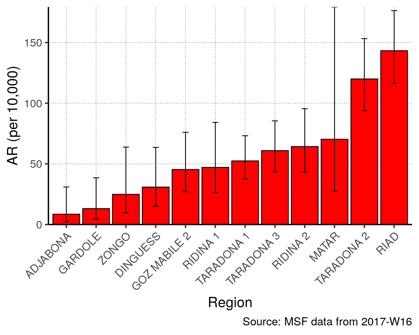
You could then also plot this on a bar chart with confidence intervals.
There are many quartiers without population denominators that will make the graph difficult to read. Thus, we modify the code by filtering ar_region to remove these using the opposite (!) of the is.na() function (see Operators R Basics page). Now any quartiers with missing denominators will not appear in the graph.
# filter ar for non-zero quartiers
ar_region <- filter(ar_region, !is.na(`AR (per 10,000)`))

# plot with the region on the x axis sorted by increasing ar
# ar value on the y axis
ggplot(ar_region, aes(x = reorder(Region, `AR (per 10,000)`),
               y = `AR (per 10,000)`)) +
  geom_bar(stat = "identity", col = "black", fill = "red") + # plot as bars (identity = as is)
  geom_errorbar(aes(ymin = `Lower 95%CI`, ymax = `Upper 95%CI`), width = 0.2) + # add CIs
  scale_y_continuous(expand = c(0,0)) +  # set origin for axes
  # add labels to axes and below chart
  labs(x = "Region", y = "AR (per 10,000)",
       captions = str_glue("Source: MSF data from {reporting_week}")) +
  epicurve_theme
You could also table mortality rate by region. A few things to note:
- The first command uses
group_by()to count cases bypatient_origin. Then,filter()is applied based on the character search functionstr_detect()from the package stringr, which looks for “Dead” within the variableexit_status- note: we must change this to reflect our data and havestr_detect()look inexit_status2(otherwise, the objectdeathshas 0 rows andmortality_rate()produces an error).
- The
mortality_rate()step calculates mortality rates for the regions that had a death.
deaths <- group_by(linelist_cleaned, patient_origin) %>%
  filter(str_detect(exit_status2, "Dead")) %>%
  summarise(deaths = n()) %>% # count deaths by region
  left_join(population_data_region, by = "patient_origin") # merge population data

mortality_rate(deaths$deaths, deaths$population, multiplier = 10000) %>%
  # add the region column to table
  bind_cols(select(deaths, patient_origin), .) %>%
  merge_ci_df(e = 4) %>% # merge the lower and upper CI into one column
  rename("Region" = patient_origin,
         "Deaths" = deaths,
         "Population" = population,
         "Mortality (per 10,000)" = `mortality per 10 000`,
         "95%CI" = ci) %>%
kable(digits = 1)| Region | Deaths | Population | Mortality (per 10,000) | 95%CI |
|---|---|---|---|---|
| ABLELAYE | 1 | - | - | (NA–NA) |
| AL-HOUGNA | 1 | - | - | (NA–NA) |
| AMSINENE | 1 | - | - | (NA–NA) |
| ANFANDOCK | 1 | - | - | (NA–NA) |
| BADINA | 1 | - | - | (NA–NA) |
| DELEBAE | 1 | - | - | (NA–NA) |
| DINGUESS | 1 | 2268 | 4.4 | (0.78–24.93) |
| GOZ MABILE | 1 | - | - | (NA–NA) |
| HARAZA | 1 | - | - | (NA–NA) |
| KACHKACHA | 2 | - | - | (NA–NA) |
| MINA | 1 | - | - | (NA–NA) |
| RIAD | 1 | 6073 | 1.6 | (0.29–9.32) |
| TARADONA 2 | 1 | 5250 | 1.9 | (0.34–10.78) |
Maps
Mapping in R can be intimidating at first because it is different than ArcGIS, QGIS, or other mapping software that primarily use a point-and-click interface. However, you will see that using commands to create maps can be much faster, more replicable, and transparent for whomever you share code with.
We do have shapefiles for the Am Timan exercise. You can download them from the case study overview page of this website.
Shapefiles are a format for storing geometric location and attribute data for geographic features - for example either points (e.g. GPS points of cases or households surveyed), lines (e.g. road network), or polygons (e.g. district boundaries)
A shapefile is actually made of several files. Viewing the shapefile in your computer’s internal folders you will often see 4 or 5 files with the same name but different extensions (e.g. .shp, .prj, etc.). As long as these files are located in the same folder the shapefile will load correctly when you import with the .shp extension.
Because we have shapefiles for this exercise, we must delete the command that generates the fake shapefile (map <- gen_polygon(regions = unique(linelist_cleaned$patient_origin))).
Note the checklist for using shapefiles:
- Your shapefile can be a polygon or points (and polygons do not have to be contiguous - they do not have to touch each other)
- Ensure that the region names in the shapefile match exactly the region names in
linelist_cleaned. (in most shapefiles there is an ID or NAME variable in the spreadsheet file)
- Make sure the coordinate reference system (CRS) of the shapefile is WGS84 (this is the standard coordinate system used by most GPS systems, but it is good to ask whomever collected to data to be sure)
When giving the name of a shapefile to here(), list the file name with a .shp extension.
The import() function is wrapped around the here() function. The here() function makes it easy for R to locate files on your computer. It is best to save the dataset within your R project, and to provide here() with any R project subfolder names. You can read more about the here() function in the data import R Basics page.
## reading in a shapefile
map <- read_sf(here::here("Quartiersshape.shp"))
The next code will check the coordinate reference system (CRS) of the shapefile, as it was read-in. In our exercise, we see an EPSG code of 4326, which is the correct code for WGS84 (you can also see below the EPSG code that the datum is WGS84).
## check the coordinate reference system (CRS)
st_crs(map)## Coordinate Reference System:
## User input: 4326
## wkt:
## GEOGCS["GCS_WGS_1984",
## DATUM["WGS_1984",
## SPHEROID["WGS_84",6378137,298.257223563]],
## PRIMEM["Greenwich",0],
## UNIT["Degree",0.017453292519943295],
## AUTHORITY["EPSG","4326"]]If there is no CRS specified for your shapefile, you can set the CRS to WGS84 with the following command, which uses the EPSG code of 4326.
## set the CRS if not present using EPSG value
## this is the most commonly used
map <- st_set_crs(map, value = 4326) # Sets to WGS84
Below we explain each step within the this code chunk, plotting a map based on the attack rate table.
Create a categorical variable of the attack rate. These categories will appear in the map as the legend - and the regions will be colored by these groups.
The first command defines
max_aras the highest attack rate value in the objectar. This is referenced later.In the next command,
breakersis defined as a sequence of integers. Zero is included by default because it should be a separate color on the final map. After zero, quartiles are determined up to themax_ar.In the last command,
mutate()is used to makear_map(a copyar_region), and add thecategoriesvariable. This variable is created usingbreakersto define the breaks in the numeric variableAR (per 10,000).
## create a categorical variable for plotting
max_ar    <- max(ar_region$`Upper 95%CI`, na.rm = TRUE) # define your highest AR

breakers <- as.integer(c(
                         # include zero as a standalone group
                         0,
                         # 1 to 4 divisions, snapping the boundaries to the nearest 100
                         find_breaks(n = max_ar, breaks = 4, snap = 100)
             ))

## add a categorical variable using the age_categories function
## nb in this case we arent using ages - but it functions the same way!
ar_map <- mutate(ar_region,
             categories = age_categories(`AR (per 10,000)`,
                                         breakers = breakers)
             )
Join the object map (shapefile) to ar_map (a data frame). The spatial object map is joined to the data frame ar_map with a left join (see the Advanced R Basics page to learn more about joins). Both of these objects contain tables (you can click them in the Environment pane to see this). In the command, they are linked by the Name variable in ar and the Region variable in map.
You may need to modify your code so that the join occurs on Name in the object map, and not name.
Make sure you modify your left_join code to use “Name” with a capital N, as that is how the variable is spelled in the object ‘map’. In your other data these variable names may be completely different and must be changed
The resulting object mapsub is a product of this left join. A left join will include all values from the Left-hand Side (LHS) and only inlcude values from the Right-hand Side (RHS) if they match to LHS values. Now, the attack rates are joined to the region names and to their GIS geometries. You can verify this by Viewing the object mapsub (click on it in the Environment pane).
## join your ar or case counts based on matching shapefile names with regions in your ar table
mapsub <- left_join(map, ar_map, by = c("Name" = "Region"))
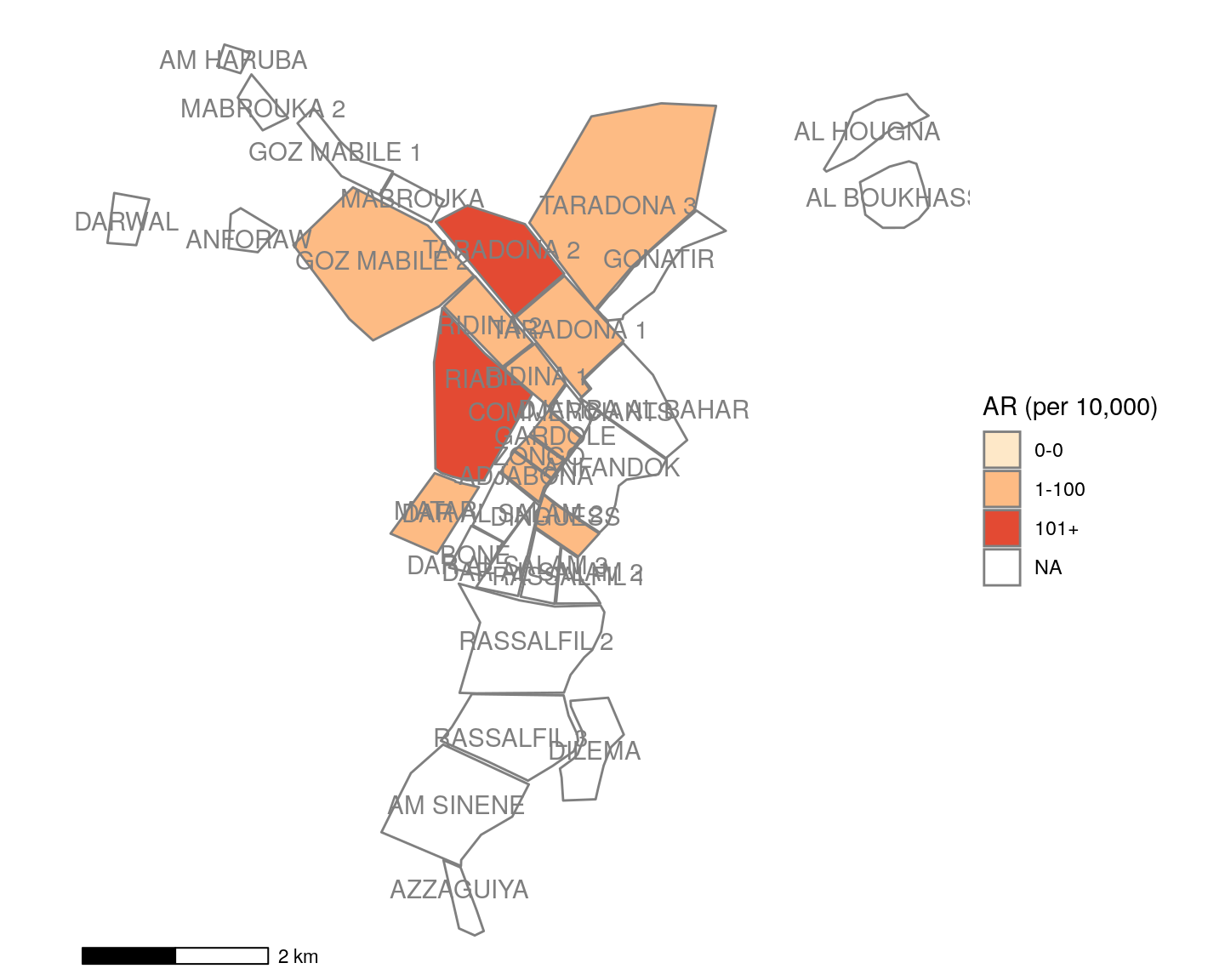
Now, ggplot() is used to create the map. Remember that ggplot() subcommands must be connected by plus symbols at the end of each line (+) (except the last line). Read more about ggplot2 and ggplot() in the Advanced R Basics page.
geom_sf() identifies mapsub as providing the data for the map, and filling the polygons by values in the variable categories.
coord_sf() set to NA prevents gridlines from being drawn on the map.
annotation_scale() adds a scalebar at the bottom of the map.
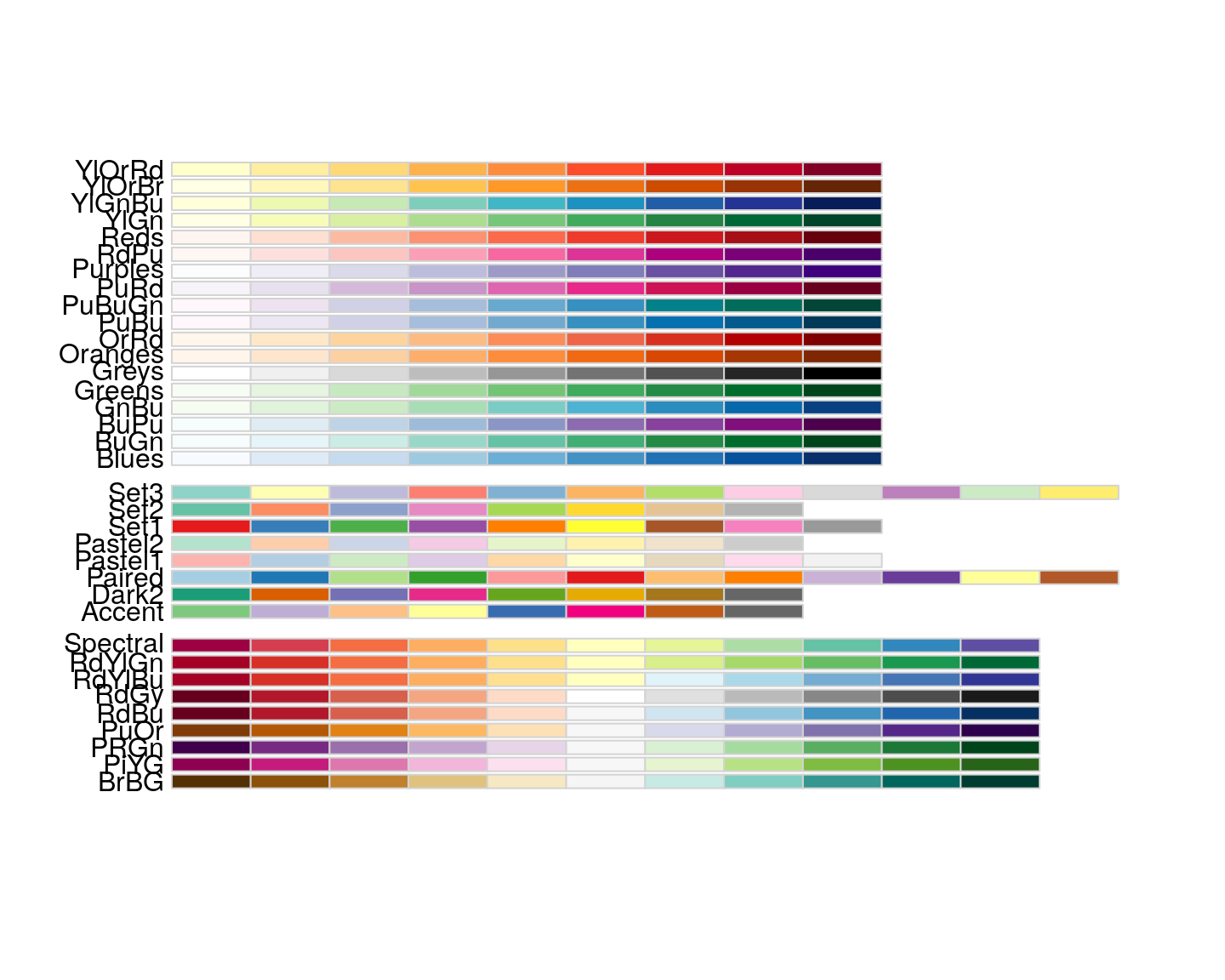
scale_fill_brewer() uses a color palatte from orange to red (“OrRd”), keeps all color levels even if there are no polygons at that level (drop=FALSE), and specifies a title for the legend. If you want a different color scale, use this code from the package RColorBrewer to see the possible options (hint: after running this code click “Zoom” in your Plot/Viewer pane to see more clearly). Then replace “OrRd” with your desired code. You can read more about colors here.
library(RColorBrewer)
display.brewer.all()
geom_sf_text() specifies labels for the polygons, including which variable to use for labels (Name), and the text colour. Again, we need to modify this ggplot() reference to the variable “name” to now reference “Name” with a capital N. In your other data the variable may be completely different.
theme_void() specifies a theme for the map that does not include coordinates or axes.
## plotting with polygons ------------------------------------------------------

ggplot() +
  geom_sf(data = mapsub, aes(fill = categories), col = "grey50") + # shapefile as polygon
  coord_sf(datum = NA) + # needed to avoid gridlines being drawn
  annotation_scale() + # add a scalebar
  scale_fill_brewer(drop = FALSE, palette = "OrRd", name = "AR (per 10,000)") +
  geom_sf_text(data = mapsub, aes(label = Name), colour = "grey50") + # label polygons
  theme_void() # remove coordinates and axes
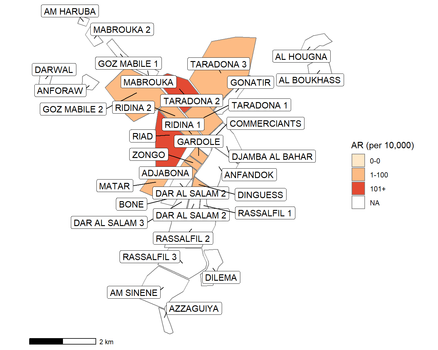
You can use this alternative to make the labels not overlap.
ggrepel() arranges point/polygon labels so they do not overlap and are easier to read. You can see more examples of ggrepel() in this vignette
The geom_sf_text() line has been replaced by ggrepel.
## plotting with polygons ------------------------------------------------------

ggplot() +
  geom_sf(data = mapsub, aes(fill = categories), col = "grey50") + # shapefile as polygon
  coord_sf(datum = NA) + # needed to avoid gridlines being drawn
  annotation_scale() + # add a scalebar
  scale_fill_brewer(drop = FALSE, palette = "OrRd", name = "AR (per 10,000)") +

  # Optional ggrepel section to make labels appear more nicely
  ggrepel::geom_label_repel(data = mapsub, aes(label = Name, geometry = geometry),
                            stat = "sf_coordinates",
                            min.segment.length = 0) +

  theme_void()  # remove coordinates and axes
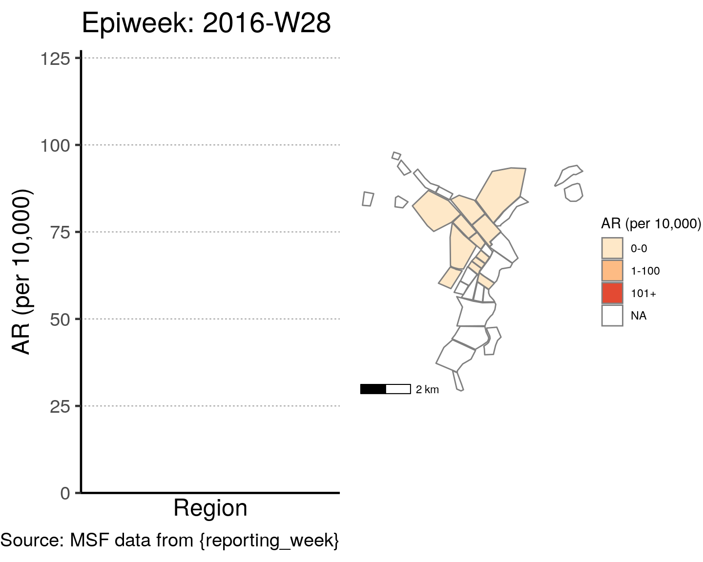
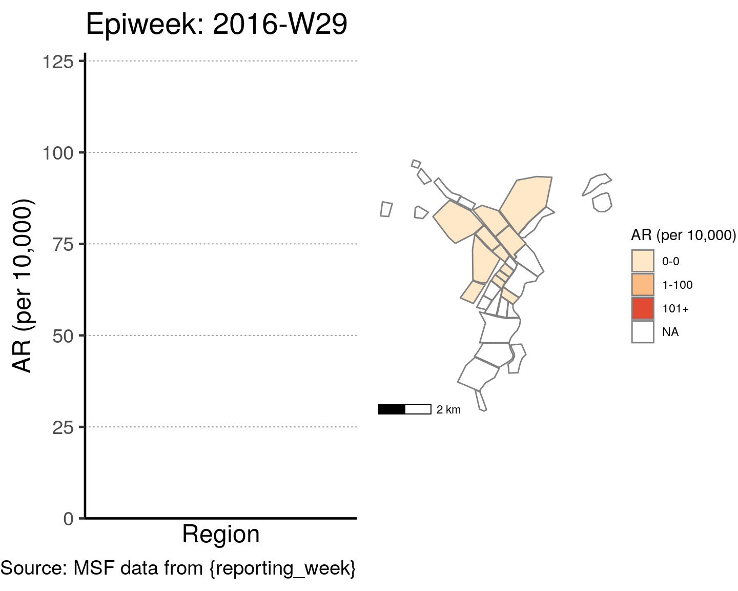
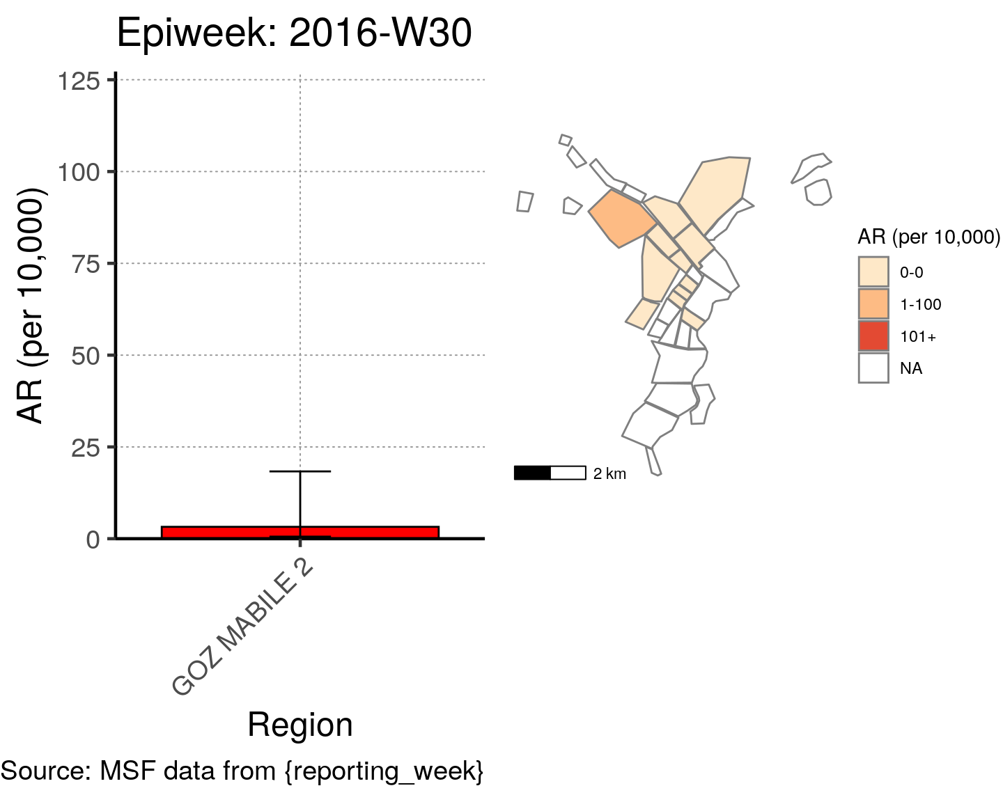
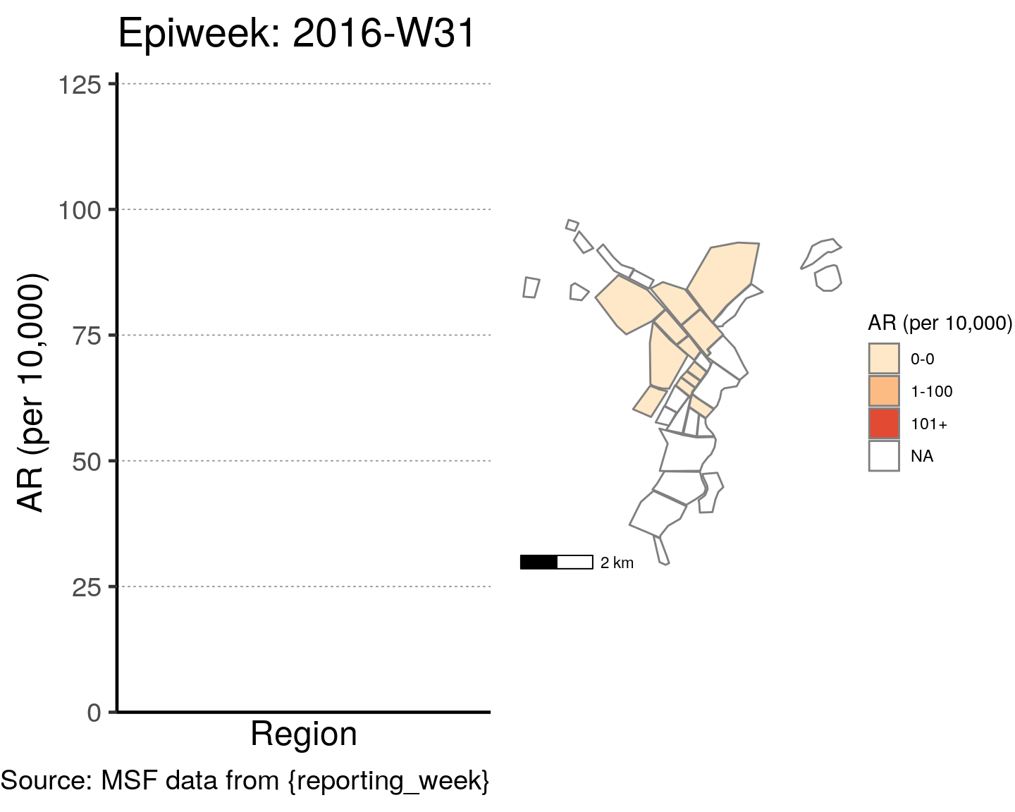
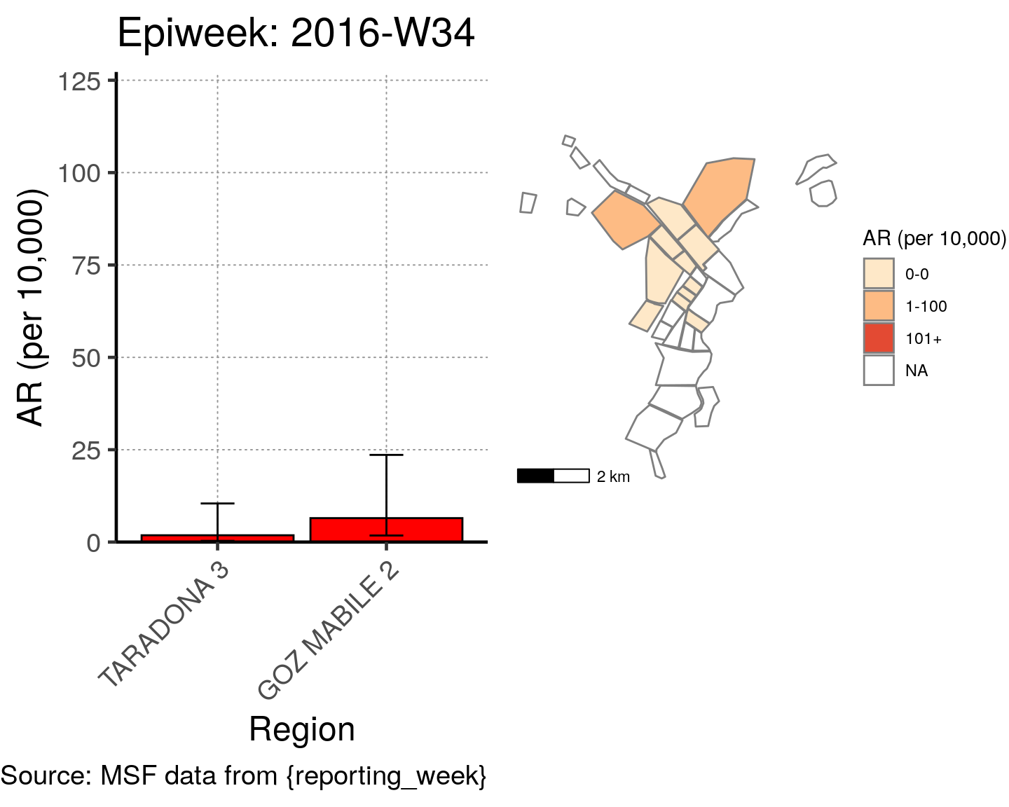
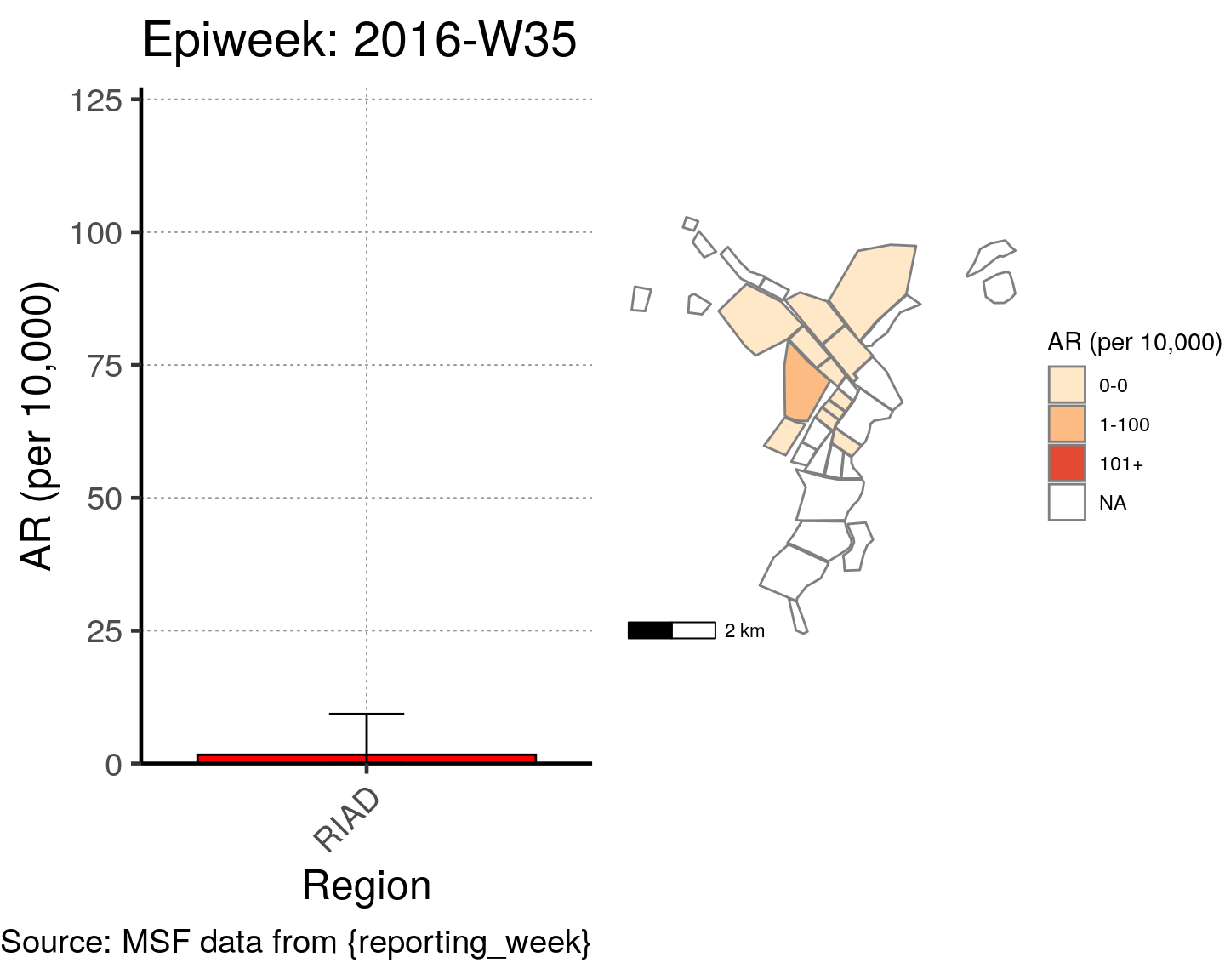
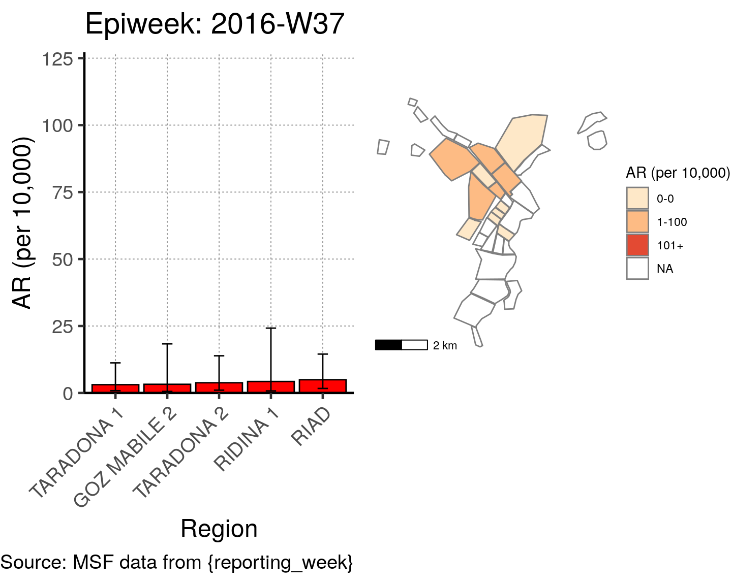
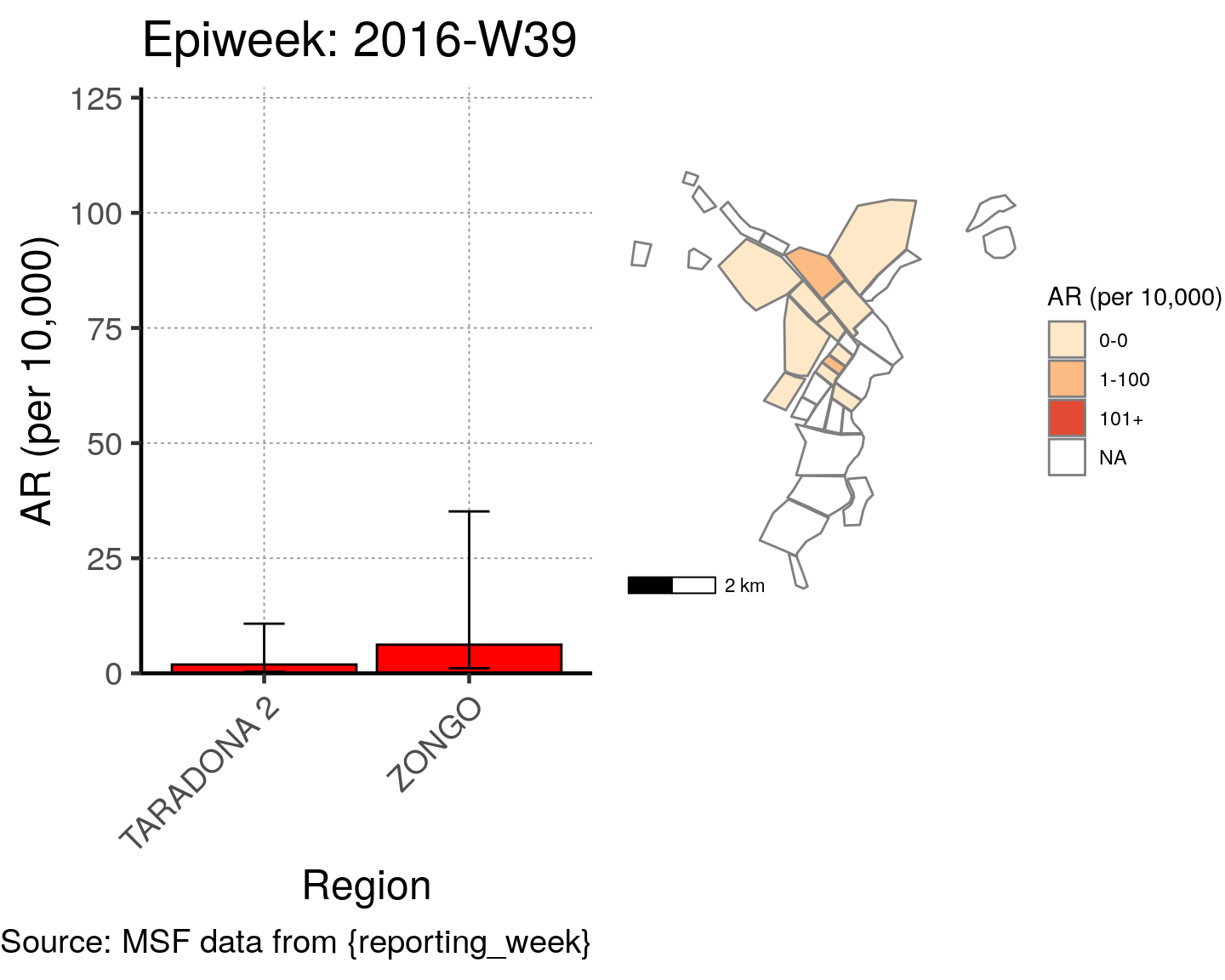
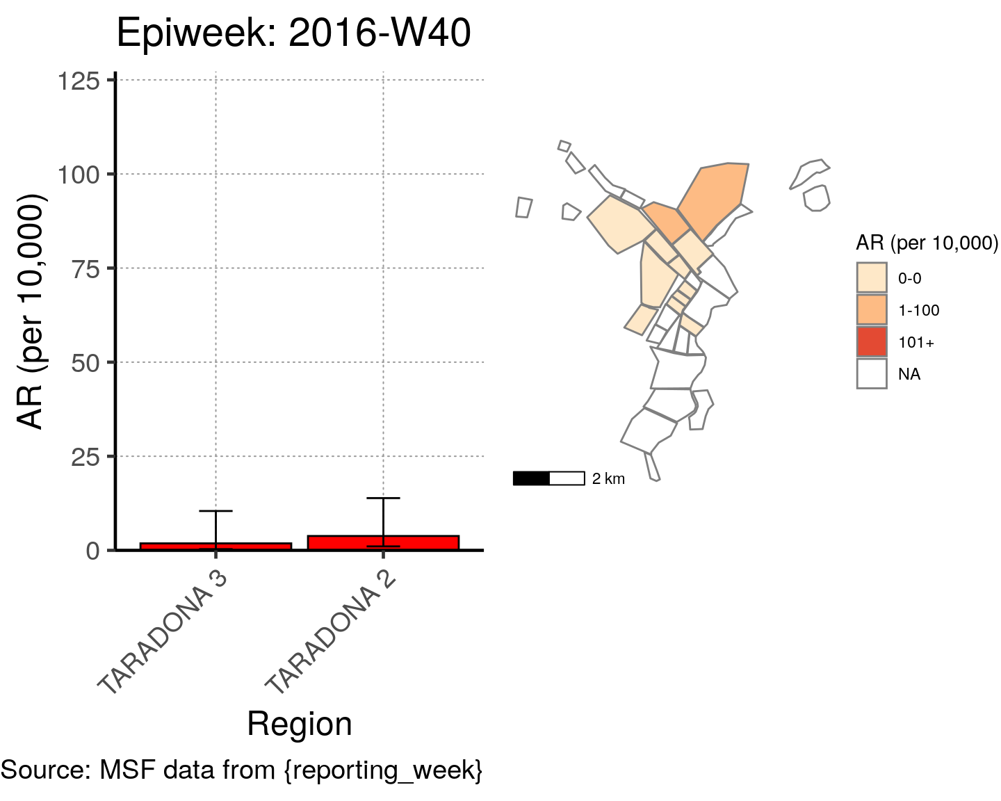
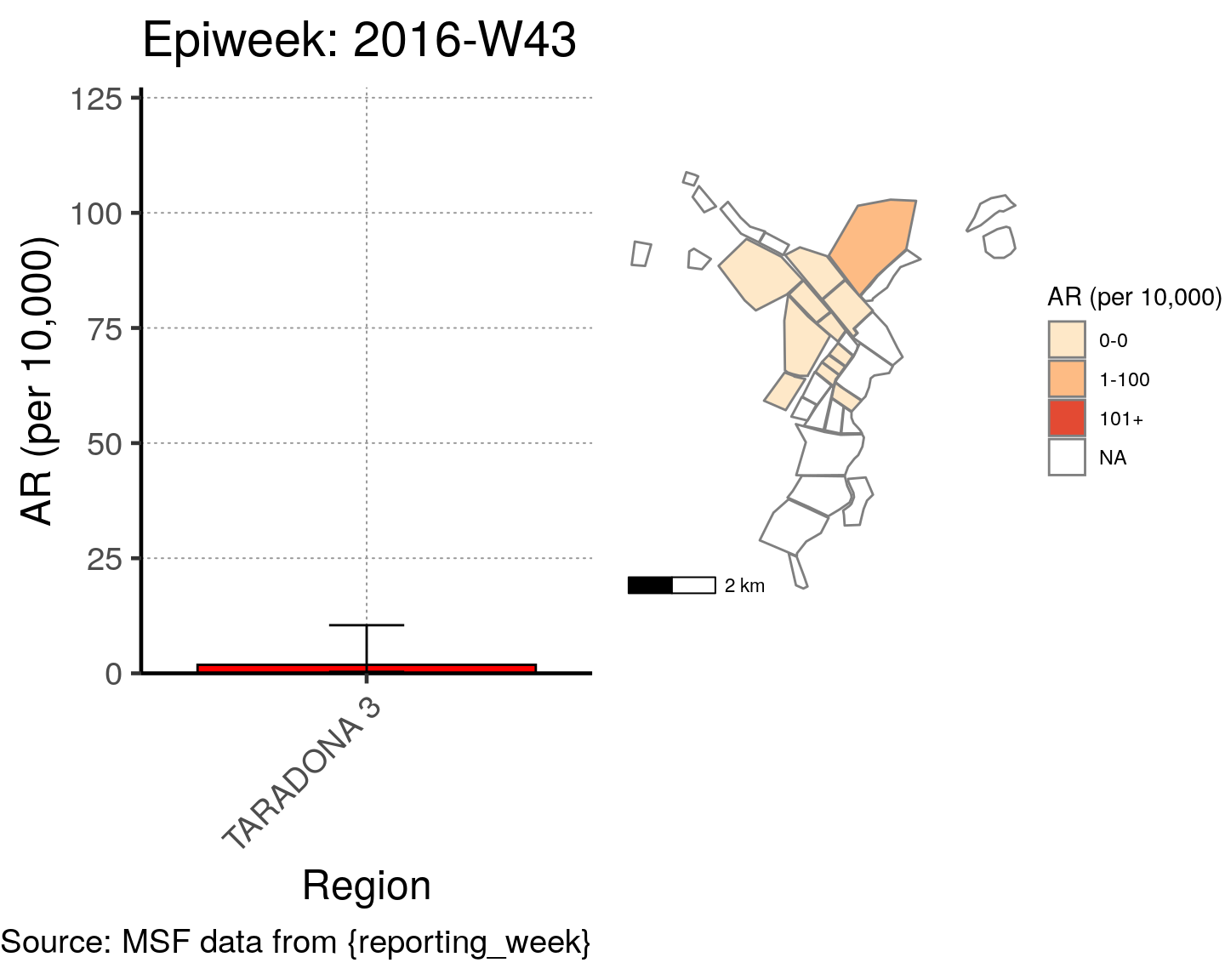
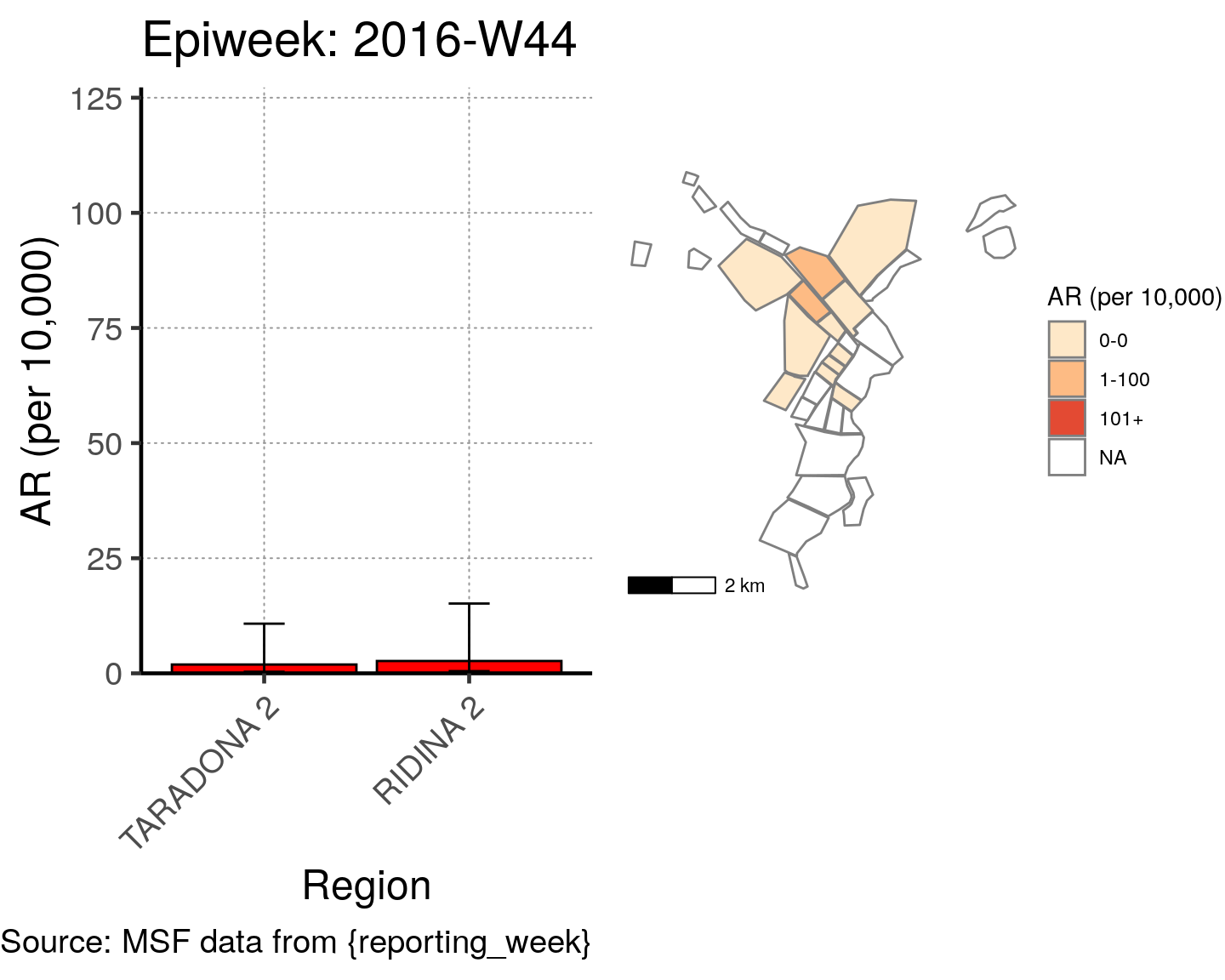
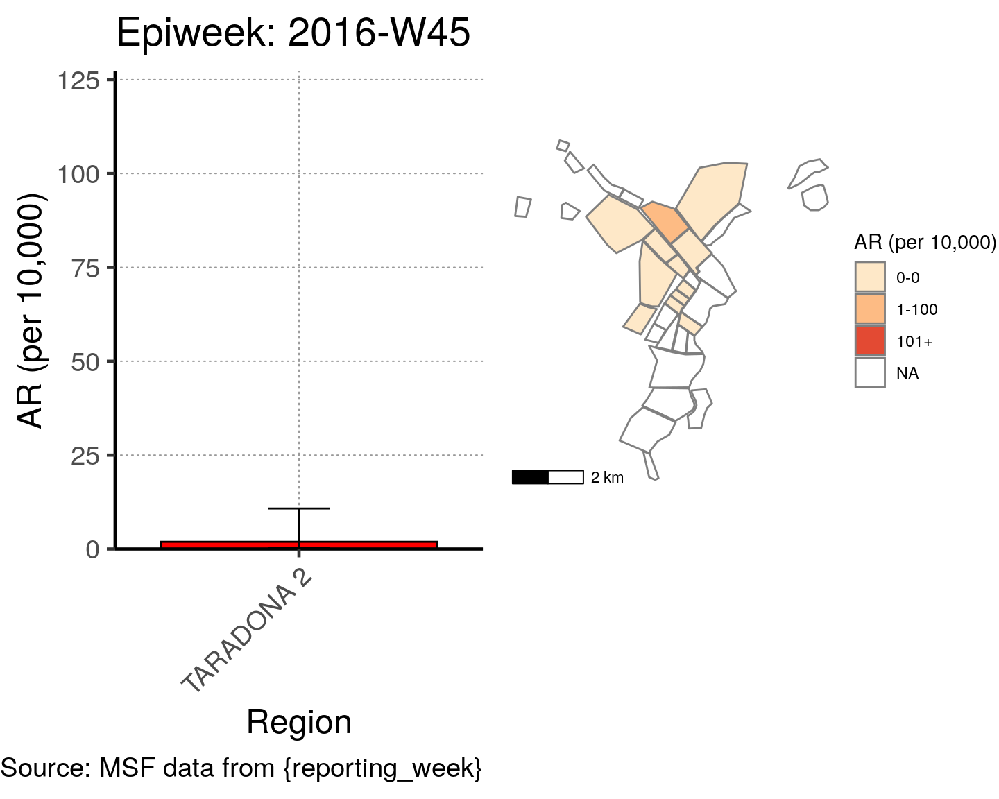
Lastly, there is an efficient way to create attack rate maps and bar plots of incidence for each epiweek. Use a “for loop” to run the same code for every epi week.
A “for loop”" is used to iterate over (perform the same actions to) every value in a vector. In this case, we want to make the map and bar chart for each region. You can read more about for loops in the R Basics - Advanced and Miscellaneous page, or this tutorial.
A few things to note about this chunk:
- The first half is very similar to the set-up of the previous map.
- You must also modify the
left_joincommand to list the correct variable names (e.g. modify to join onNameinstead ofname) - These maps are not labeled with region names.
- The creation of the barplots depends on the object
epicurve_theme, which was defined in the Time section of the template. If that section is not created, then this object will be missing and cause errors.
The barplots can be limited to quartiers with non-zero attack rates with the following code:
  # Filter values in this_ar to only show quartiers with attack rates > 0 in barplot
  this_ar <- filter(this_ar, `AR (per 10,000)` > 0)
And here is the complete code:
## Checklist for plotting in for-loop ------------------------------------------
## - [ ] decide if you would like to show counts, AR or categories of those
## - [ ] define appropriate breaks to ensure legend is uniform by week
## - [ ] replace `Cases (n)` and `AR (per 10,000)` or "categories", appropriately
## - [ ] consider facet wrapping by an overarching unit if have many regions (e.g. by province)

# change region variable to a factor so that zero counts can be included
linelist_cleaned$patient_origin <- as.factor(linelist_cleaned$patient_origin)

# case counts
cases <- linelist_cleaned %>%
  group_by(epiweek) %>%
  count(patient_origin, .drop = FALSE) %>%   # cases for each week by region
  left_join(population_data_region, by = "patient_origin")    # merge population data

# attack rate for region
ar <- attack_rate(cases$n, cases$population, multiplier = 10000) %>%
  # add the region column to table
  bind_cols(select(cases, epiweek, patient_origin), .) %>%
  rename("Region" = patient_origin,
         "Cases (n)" = cases,
         "Population" = population,
         "AR (per 10,000)" = ar,
         "Lower 95%CI" = lower,
         "Upper 95%CI" = upper)
max_cases <- max(cases$n, na.rm = TRUE) # define the maximum number of cases for the color palette
max_ar    <- max(ar$`Upper 95%CI`, na.rm = TRUE)

## define breaks for standardising color palette
breakers <- as.integer(c(
                         # include zero as a standalone group
                         0,
                         # 1 to 4 divisions, snapping the boundaries to the nearest 100
                         find_breaks(n = max_ar, breaks = 4, snap = 100)
             ))

## add a categorical variable using the age_categories function
## nb in this case we arent using ages - but it functions the same way!
ar <- mutate(ar,
             categories = age_categories(`AR (per 10,000)`,
                                         breakers = breakers)
             )
Note: Only results for the first 20 epiweeks are shown. Also, the barplots are filtered to only show quartiers with non-zero attack rates.
# All the code is contained within a FOR LOOP that goes through each epiweek, filters and plots the data

for (i in unique(cases$epiweek)) {

  # filters the large ar dataframe for the epiweek being examined ("i")
  this_ar <- filter(ar, epiweek == i)

  ### Create Map for epiweek "i"
  # map
  mapsub <- left_join(map, this_ar, by = c("Name" = "Region"))

  # choropleth
  map_plot <- ggplot() +
    geom_sf(data = mapsub, aes(fill = categories), col = "grey50") + # shapefile as polygon
    coord_sf(datum = NA) + # needed to avoid gridlines being drawn
    annotation_scale() + # add a scalebar
  scale_fill_brewer(drop = FALSE,
                    palette = "OrRd",
                    name = "AR (per 10,000)") +  # color the scale to be perceptually uniform (keep levels)
    theme_void() # remove coordinates and axes

  ### Create barplot for epiweek "i"

  # Filter values in this_ar to only show quartiers with attack rates > 0 in barplot
  this_ar <- filter(this_ar, `AR (per 10,000)` > 0)

  # Create barplot for epiweek "i"
  barplot <- ggplot(this_ar, aes(x = reorder(Region, `AR (per 10,000)`),
                                 y = `AR (per 10,000)`)) +
    geom_bar(stat = "identity", col = "black", fill = "red") + # plot as bars (identity = as is)
    geom_errorbar(aes(ymin = `Lower 95%CI`, ymax = `Upper 95%CI`), width = 0.2) + # add CIs
    scale_y_continuous(expand = c(0, 0), limits = c(0, max_ar)) +  # set origin for axes
    # add labels to axes and below chart
    labs(x = "Region", y = "AR (per 10,000)",
         captions = ("Source: MSF data from {reporting_week}")) +
    epicurve_theme


  # combine the barplot and map plot into one for epiweek "i"
  print(
    cowplot::plot_grid(
      barplot + labs(title = str_glue("Epiweek: {i}")),
      map_plot,
      nrow = 1,
      align = "h",
      axis = "tb"
    )
  )
}