First steps
Opening a new R project
Please review the instructions in the R Basics page on Working within R projects. In brief:
Open RStudio. Select New Project from the main File menu of RStudio. Select New Directory and New Project, and a location to save the new R project (this creates a new folder).
Save all relevant data files into this new R project folder.
For the RMarkdown to produce the final report correctly, you must have read/write permissions for the location of the R project folder. On an MSF computer this is generally the c:/temp folder.
Opening an AJS template
Once the R project is established,
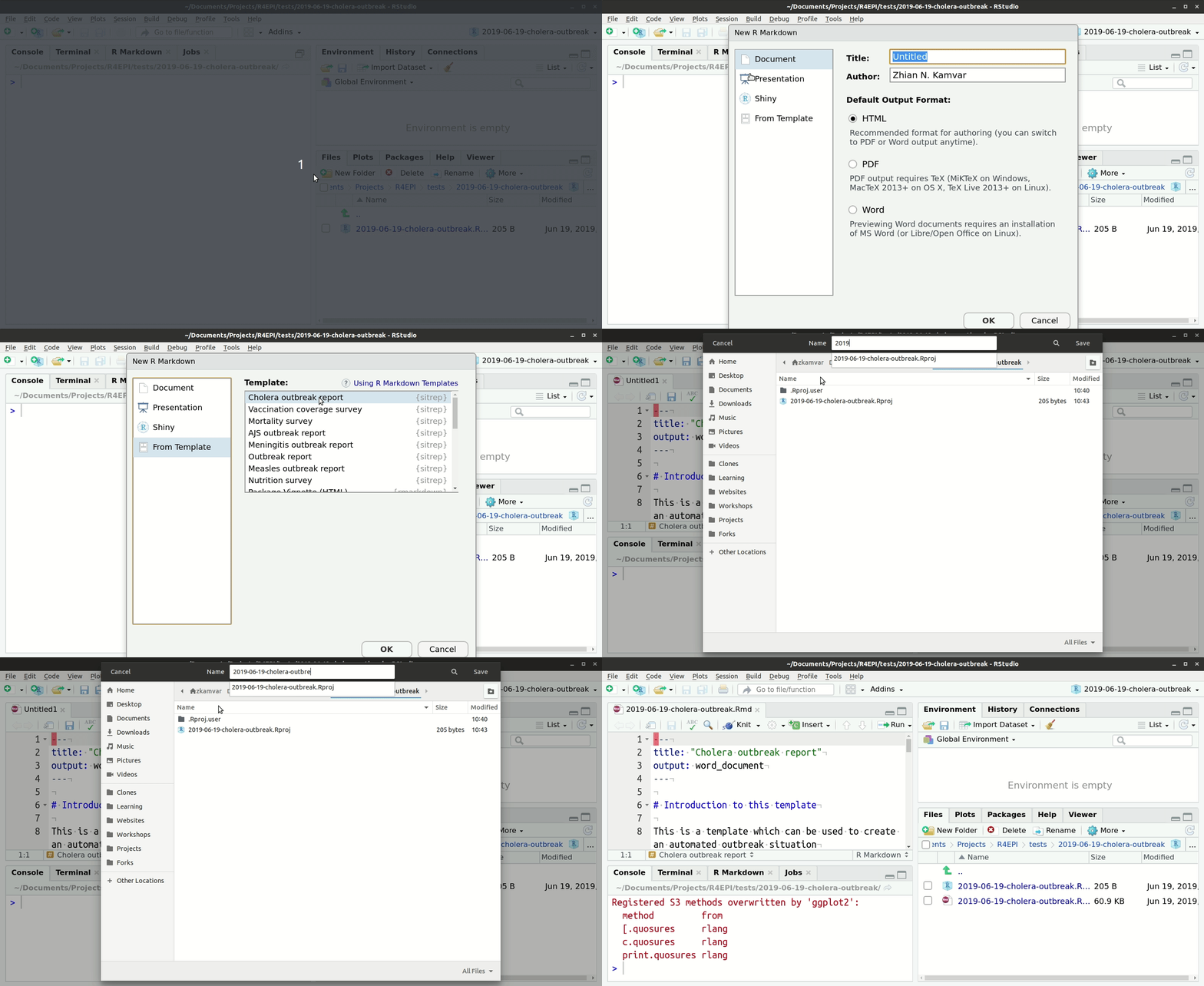
- Select New File from the main File menu of RStudio, and select “R Markdown”
- In the pop-up window, select From Template on the right side
- Then select AJS outbreak report from the menu on the right
The AJS RMarkdown template will open in your RStudio Viewer pane.
Below is an example showing how to open and save an outbreak template. Be sure to open the AJS template for this exercise.
Now, follow along with this walk-through and make edits to your AJS template, saving it regularly.
Header
The very top of the template consists of a header surrounded by --- lines. Here you may want to edit the title of your document. The other settings in the header define the default document type produced (Microsoft Word) when the RMarkdown is “knit”.
Remember that the green text below the header, located between these special characters (<!-- and -->), is for your information only. This text will not appear in the final Word document report (see the R Basics page Reading a RMarkdown for more information).
Introduction to the template
This text just below the header is for your reference only. If left alone it will appear at the beginning of your report, so you should replace it with a more relevant introduction. Any text you write here can be formatted with italics, bold, bullets, numbers, tables, and in-line code. See this RMarkdown cheatsheet for tips on formatting.
Installing and loading packages
The first code chunk, setup, is very important and must be kept. When the final report is knit, this chunk will run without producing any output, but it is required for the template to work correctly.
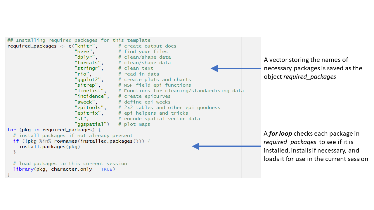
This setup code chunk does the following:
Set default settings for tables such as size, error handling, and display of missing values
Create a vector of names of packages required for the template to run
Execute a for loop to install each required package (if not already installed), and load each required package for use in the current R session (learn about for loops in the R Basics Advanced and Miscellaneous page.
Set default text size in graphic plots
Establish visual theme settings for epidemic curve plots
About the packages used in this template
Generic packages
- knitr used to create the output document (pdf, doc, html)
- dplyr used to clean and shape the data
- forcats used to clean and shape the data
- stringr used to clean and handle text/characters (known in computer science as “strings”)
- rio used to read in data
- ggplot2 used to visualise your data using different plotting methods
- here used to locate files
More epidemiology-specific packages
- sitrep includes a variety of useful field epidemiology functions
- linelist used for cleaning and standardising data
- incidence used for creating epicurves
- aweek used for creating epiweeks
- epitools used for creating 2by2 tables
- epitrix used for helpful epidemiological tasks
Mapping packages
- ggspatial used for selecting basemap tiles
- sf used for manipulating spatial objects (e.g. polygons) easily
Define current epi week
This chunk continues the set-up of time-related parameters.
First, ensure epidemiological weeks are set to begin on Mondays using the function set_week_start() from the package aweek. See the documentation of the package aweek for more information.
Second, set the reporting week for the report. This value is used in later code chunks, for example when producing epidemic curves. Note that you likely want to specify the most recent complete epi week. Follow the format in the code below (within quotes give the 4-digit year, a hyphen (-), capital W, then the 2-digit epi week number).
To determine which epi week of a date you can use the date2week() function. It will tell you the year, week, and day number of the provided date. Let’s assume the date of this analysis is 27 April, 2017, so the most recent complete epidemiological week is Week 16 of 2017.
aweek::date2week("2017-04-27") # Ask for the epi week of this date## <aweek start: Monday>
## [1] "2017-W17-4"reporting_week <- aweek::as.aweek("2017-W16") # Set reporting_week as last complete epi weekIf you want to use the automatically-updated date from your computer, use Sys.Date() like this: date2week(Sys.Date())
Lastly, the labels that will be used in epidemic curve plots are defined. These should not need any adjustment. You may notice that the subtitle label uses reporting_week in curly braces—this means that the value of reporting_week defined in the previous chunk will show in its place.
## sets the labels in ggplot for the epicurves
epicurve_labels <- labs(x = "Calendar week",
                        y = "Cases (n)",
                        title = "Cases by week of onset",
                        subtitle = str_glue("Source: MSF data from {reporting_week}")
) 

